Overview#

After compiling ASPECT as described above, you should have an executable file in the build directory. It can be called in the build directory as follows:

  ./aspect parameter-file.prm

or, if you want to run the program in parallel, using something like

  mpirun -np 4 ./aspect parameter-file.prm

to run with 4 processors. In either case, the argument denotes the (path and) name of a file that contains input parameters.[1] When you download ASPECT, there are a number of sample input files in the cookbooks directory, corresponding to the examples discussed in Cookbooks, and input files for some of the benchmarks discussed in Benchmarks are located in the benchmarks directory. A full description of all parameters one can specify in these files is given in Parameter Documentation.

Running ASPECT with an input file[2] will produce output that will look something like this (numbers will all be different, of course):

-----------------------------------------------------------------------------
-- This is ASPECT, the Advanced Solver for Problems in Earth's ConvecTion.
--     . version 2.0.0-pre (include_dealii_version, c20eba0)
--     . using deal.II 9.0.0-pre (master, 952baa0)
--     . using Trilinos 12.10.1
--     . using p4est 2.0.0
--     . running in DEBUG mode
--     . running with 1 MPI process
-----------------------------------------------------------------------------

Number of active cells: 1,536 (on 5 levels)
Number of degrees of freedom: 20,756 (12,738+1,649+6,369)

*** Timestep 0:  t=0 years

   Rebuilding Stokes preconditioner...
   Solving Stokes system... 30+3 iterations.
   Solving temperature system... 8 iterations.

Number of active cells: 2,379 (on 6 levels)
Number of degrees of freedom: 33,859 (20,786+2,680+10,393)

*** Timestep 0:  t=0 years

   Rebuilding Stokes preconditioner...
   Solving Stokes system... 30+4 iterations.
   Solving temperature system... 8 iterations.

   Postprocessing:
     Writing graphical output: output/solution/solution-00000
     RMS, max velocity:        0.0946 cm/year, 0.183 cm/year
     Temperature min/avg/max:  300 K, 3007 K, 6300 K
     Inner/outer heat fluxes:  1.076e+05 W, 1.967e+05 W

*** Timestep 1:  t=1.99135e+07 years

   Solving Stokes system... 30+3 iterations.
   Solving temperature system... 8 iterations.

   Postprocessing:
     Writing graphical output: output/solution/solution-00001
     RMS, max velocity:        0.104 cm/year, 0.217 cm/year
     Temperature min/avg/max:  300 K, 3008 K, 6300 K
     Inner/outer heat fluxes:  1.079e+05 W, 1.988e+05 W

*** Timestep 2:  t=3.98271e+07 years

   Solving Stokes system... 30+3 iterations.
   Solving temperature system... 8 iterations.

   Postprocessing:
     RMS, max velocity:       0.111 cm/year, 0.231 cm/year
     Temperature min/avg/max: 300 K, 3008 K, 6300 K
     Inner/outer heat fluxes: 1.083e+05 W, 2.01e+05 W

*** Timestep 3:  t=5.97406e+07 years

...

The output starts with a header that lists the used ASPECT, deal.II, Trilinos and p4est versions as well as the mode you compiled ASPECT in (see Debug or optimized mode), and the number of parallel processes used.[3] With this information we strive to make ASPECT models as reproducible as possible.

The following output depends on the model, and in this case was produced by a parameter file that, among other settings, contained the following values (we will discuss many such input files in Cookbooks:

set Dimension                     = 2
set End time                      = 1.5e9
set Output directory              = output

subsection Geometry model
  set Model name                  = spherical shell
end

subsection Mesh refinement
  set Initial global refinement   = 4
  set Initial adaptive refinement = 1
end

subsection Postprocess
  set List of postprocessors      = visualization, velocity statistics, temperature statistics, heat flux statistics, depth average
end

In other words, these run-time parameters specify that we should start with a geometry that represents a spherical shell (see Geometry model and Subsection: Geometry model / Spherical shell for details). The coarsest mesh is refined 4 times globally, i.e., every cell is refined into four children (or eight, in 3d) 4 times. This yields the initial number of 1,536 cells on a mesh hierarchy that is 5 levels deep. We then solve the problem there once and, based on the number of adaptive refinement steps at the initial time set in the parameter file, use the solution so computed to refine the mesh once adaptively (yielding 2,379 cells on 6 levels) on which we start the computation over at time $t=0$.

Within each time step, the output indicates the number of iterations performed by the linear solvers, and we generate a number of lines of output by the postprocessors that were selected (see Postprocess). Here, we have selected to run all postprocessors that are currently implemented in ASPECT which includes the ones that evaluate properties of the velocity, temperature, and heat flux as well as a postprocessor that generates graphical output for visualization.

While the screen output is useful to monitor the progress of a simulation, its lack of a structured output makes it not useful for later plotting things like the evolution of heat flux through the core-mantle boundary. To this end, ASPECT creates additional files in the output directory selected in the input parameter file (here, the output/ directory relative to the directory in which ASPECT runs). In a simple case, this will look as follows:

aspect> ls -l output/
total 932
-rw-rw-r-- 1 bangerth bangerth  11134 Dec 11 10:08 depth_average.gnuplot
-rw-rw-r-- 1 bangerth bangerth  11294 Dec 11 10:08 log.txt
-rw-rw-r-- 1 bangerth bangerth     42 Dec 11 10:07 original.prm
-rw-rw-r-- 1 bangerth bangerth 326074 Dec 11 10:07 parameters.prm
-rw-rw-r-- 1 bangerth bangerth 577138 Dec 11 10:07 parameters.tex
drwxr-xr-x 2 bangerth bangerth   4096 Dec 11 10:08 solution
-rw-rw-r-- 1 bangerth bangerth    484 Dec 11 10:08 solution.pvd
-rw-rw-r-- 1 bangerth bangerth    451 Dec 11 10:08 solution.visit
-rw-rw-r-- 1 bangerth bangerth   8267 Dec 11 10:08 statistics

The purpose of these files is as follows:

Screen output: The file output/log.txt contains a copy of the output that is printed to the terminal when you run ASPECT.
A listing of all run-time parameters: The file output/original.prm is a copy of the parameter file that was used in this computation. It is often useful to save this file together with simulation data to allow for the easy reproduction of computations later on.

The output/parameters.prm file contains a complete listing of all run-time parameters. In particular, this includes the ones that have been specified in the input parameter file passed on the command line, but it also includes those parameters for which defaults have been used. This file can also be used to explore all available parameters and possible options as it contains the documentation of all parameters.

Finally, there is output/parameters.tex, that lists the parameters like output/parameters.prm in LaTeX format, and output/parameters.json in JSON format.

While output/parameters.prm contains all parameters (with their default values if they were not specified), all formatting and comments are lost. As output/original.prm is identical to the prm you started ASPECT with, it preserves comments and formatting while not outputting the default values (or documentation).
Graphical output files: One of the postprocessors chosen in the parameter file used for this computation is the one that generates output files that represent the solution at certain time steps. The screen output indicates that it has run at time step 0, producing output files that start with output/solution/solution-00000. Depending on the settings in the parameter file, output will be generated every so many seconds or years of simulation time, and subsequent output files will then start with output/solution/solution-00001, all placed in the output/solution subdirectory. This is because there are often a lot of output files: For many time steps, times the number of processors, so they are placed in a subdirectory so as not to make it more difficult than necessary to find the other files.

At the current time, the default is that ASPECT generates this output in VTK format[4] as that is widely used by a number of excellent visualization packages and also supports parallel visualization.[5] If the program has been run with multiple MPI processes, then the list of output files will be output/solution/solution-XXXXX.YYYY denoting that this the XXXXXth time we create output files and that the file was generated by the YYYYth processor.

VTK files can be visualized by many of the large visualization packages. In particular, the VisIt and ParaView programs, both widely used, can read the files so created. However, while VTK has become a de-facto standard for data visualization in scientific computing, there doesn’t appear to be an agreed upon way to describe which files jointly make up for the simulation data of a single time step (i.e., all files with the same XXXXX but different YYYY in the example above). VisIt and ParaView both have their method of doing things, through .pvtu and .visit files. To make it easy for you to view data, ASPECT simply creates both kinds of files in each time step in which graphical data is produced, and these are then also placed into the subdirectories as output/solution/solution-XXXXX.pvtu and output/solution/solution-XXXXX.visit.

The final two files of this kind, output/solution.pvd and output/solution.visit, are files that describes to ParaView and VisIt, respectively, which output/solution/solution-XXXXX.pvtu and output/solution/solution-XXXXX.YYYY.vtu jointly form a complete simulation. In the former case, the file lists the .pvtu files of all timesteps together with the simulation time to which they correspond. In the latter case, it actually lists all .vtu that belong to one simulation, grouped by the timestep they correspond to. To visualize an entire simulation, not just a single time step, it is therefore simplest to just load one of these files, depending on whether you use ParaView or VisIt.[6] Because loading an entire simulation is the most common use case, these are the two files you will most often load, and so they are placed in the output directory, not the subdirectory where the actual .vtu data files are located.

For more on visualization, see also Visualizing results.
A statistics file: The output/statistics file contains statistics collected during each time step, both from within the simulator (e.g., the current time for a time step, the time step length, etc.) as well as from the postprocessors that run at the end of each time step. The file is essentially a table that allows for the simple production of time trends. In the example above, and at the time when we are writing this section, it looks like this:
```
# 1: Time step number
# 2: Time (years)
# 3: Iterations for Stokes solver
# 4: Time step size (year)
# 5: Iterations for temperature solver
# 6: Visualization file name
# 7: RMS velocity (m/year)
# 8: Max. velocity (m/year)
# 9: Minimal temperature (K)
# 10: Average temperature (K)
# 11: Maximal temperature (K)
# 12: Average nondimensional temperature (K)
# 13: Core-mantle heat flux (W)
# 14: Surface heat flux (W)
0 0.000e+00 33 2.9543e+07 8                             "" 0.0000 0.0000 0.0000 0.0000    ...
0 0.000e+00 34 1.9914e+07 8 output/solution/solution-00000 0.0946 0.1829 300.00 3007.2519 ...
1 1.991e+07 33 1.9914e+07 8 output/solution/solution-00001 0.1040 0.2172 300.00 3007.8406 ...
2 3.982e+07 33 1.9914e+07 8                             "" 0.1114 0.2306 300.00 3008.3939 ...
```
The actual columns you have in your statistics file may differ from the ones above, but the format of this file should be obvious. Since the hash mark is a comment marker in many programs (for example, gnuplot ignores lines in text files that start with a hash mark), it is simple to plot these columns as time series. Alternatively, the data can be imported into a spreadsheet and plotted there.

Note

As noted in Dimensional or non-dimensionalized equations?, ASPECT can be thought of as using the meter-kilogram-second (MKS, or SI) system. Unless otherwise noted, the quantities in the output file are therefore also in MKS units.

A simple way to plot the contents of this file is shown in Visualizing statistical data.
Output files generated by other postprocessors: Similar to the output/statistics file, several of the existing postprocessors one can select from the parameter file generate their data in their own files in the output directory. For example, ASPECT’s “depth average” postprocessor will write depth-average statistics into the file output/depth_average.gnuplot. Input parameters chosen in the input file control how often this file is updated by the postprocessor, as well as what graphical file format to use (if anything other than gnuplot is desired).

By default, the data is written in text format that can be easily visualized, see for example Fig. 13. The plot shows how an initially linear temperature profile forms upper and lower boundary layers.

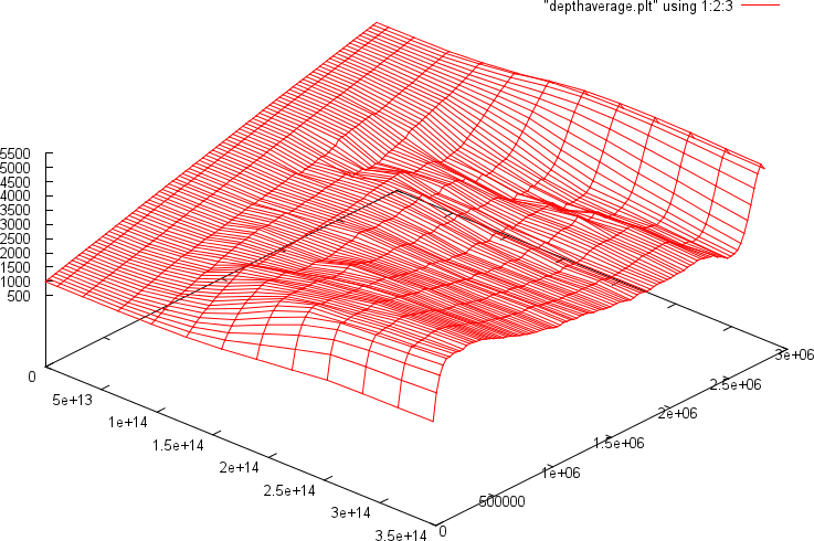
$Example output for depth average statistics. On the left axis are 13 time steps, on the right is the depth (from the top at 0 to the bottom of the mantle on the far right), and the upwards pointing axis is the average temperature. This plot is generated by gnuplot, but the depth averages can be written in many other output formats as well, if preferred (see {ref}`parameters:Postprocess/Depth_20average`).$

Fig. 13 Example output for depth average statistics. On the left axis are 13 time steps, on the right is the depth (from the top at 0 to the bottom of the mantle on the far right), and the upwards pointing axis is the average temperature. This plot is generated by gnuplot, but the depth averages can be written in many other output formats as well, if preferred (see Subsection: Postprocess / Depth average).#

There are other parts of ASPECT that may also create files in the output directory. For example, if your simulation includes advecting along particles (see Particles), then visualization information for these particles will also appear in this file. See Using particles for an example of how this looks like.

[1]

As a special case, if you call ASPECT with an argument that consists of two dashes, “--”, then the arguments will be read from the standard input stream of the program. In other words, you could type the input parameters into your shell window in this case (though that would be cumbersome, ASPECT would seem to hang until you finish typing all of your input into the window and then terminating the input stream by typing Ctrl-D). A more common case would be to use Unix pipes so that the default input of ASPECT is the output of another program, as in a command like cat parameter-file.prm.in | mypreprocessor | ./aspect --, where mypreprocessor would be a program of your choice that somehow transforms the file parameter-file.prm.in into a valid input file, for example to systematically vary one of the input parameters. If you want to run ASPECT in parallel, you can do something like cat parameter-file.prm.in | mypreprocessor | mpirun -np 4 ./aspect --. In cases like this, mpirun only forwards the output of mypreprocessor to the first of the four MPI processes, which then sends the text to all other processors.