Postprocessing spherical 3D convection

This section was contributed by Jacqueline Austermann, Ian Rose, and Shangxin Liu

There are several postprocessors that can be used to turn the velocity and pressure solution into quantities that can be compared to surface observations. In this cookbook (cookbooks/shell_3d_postprocess/shell_3d_postprocess.prm) we introduce two postprocessors: dynamic topography and the geoid. We initialize the model with a harmonic perturbation of degree 4 and order 2 and calculate the instantaneous solution. Analogous to the previous setup we use a spherical shell geometry model and a simple material model.

The relevant section in the input file that determines the postprocessed output is as follows:

subsection Postprocess
  set List of postprocessors = velocity statistics, dynamic topography, visualization, basic statistics, geoid

  subsection Visualization
    set Output format                 = vtu
    set List of output variables      = geoid, dynamic topography, density, viscosity, gravity
    set Number of grouped files       = 1
  end
end

This initial condition results in distinct flow cells that cause local up- and downwellings (Fig. 84). This flow deflects the top and bottom boundaries of the mantle away from their reference height, a process known as dynamic topography. The deflection of the surfaces and density perturbations within the mantle also cause a perturbation in the gravitational field of the planet relative to the hydrostatic equilibrium ellipsoid.

Dynamic topography at the surface and core mantle boundary.

Dynamic topography is calculated at the surface and bottom of the domain through a stress balancing approach where we assume that the radial stress at the surface is balanced by excess (or deficit) topography. We use the consistent boundary flux (CBF) method to calculate the radial stress at the surface [Zhong et al., 1993]. For the bottom surface we define positive values as up (out) and negative values are down (in), analogous to the deformation of the upper surface. Dynamic topography can be outputted in text format (which writes the Euclidean coordinates followed by the corresponding topography value) or as part of the visualization. The upwelling and downwelling flow along the equator causes alternating topography high and lows at the top and bottom surface (Fig. 84). In Fig. 84 c, d we have subtracted the mean dynamic topography from the output field as a postprocessing step outside of ASPECT. Since mass is conserved within the Earth, the mean dynamic topography should always be zero, however, the outputted values might not fulfill this constraint if the resolution of the model is not high enough to provide an accurate solution. This cookbook only uses a refinement of 2, which is relatively low resolution.

Geoid anomalies.

Geoid anomalies are perturbations of the gravitational equipotential surface that are due to density variations within the mantle as well as deflections of the surface and core mantle boundary. The geoid anomalies are calculated using a spherical harmonic expansion of the respective fields. The user has the option to specify the minimum and maximum degree of this expansion. By default, the minimum degree is 2, which conserves the mass of the Earth (by removing degree 0) and chooses the Earth’s center of mass as reference frame (by removing degree 1). In this model, downwellings coincide with lows in the geoid anomaly. That means the mass deficit caused by the depression at the surface is not fully compensated by the high density material below the depression that drags the surface down. The geoid postprocessor uses a spherical harmonic expansion and can therefore only be used with the 3D spherical shell geometry model.

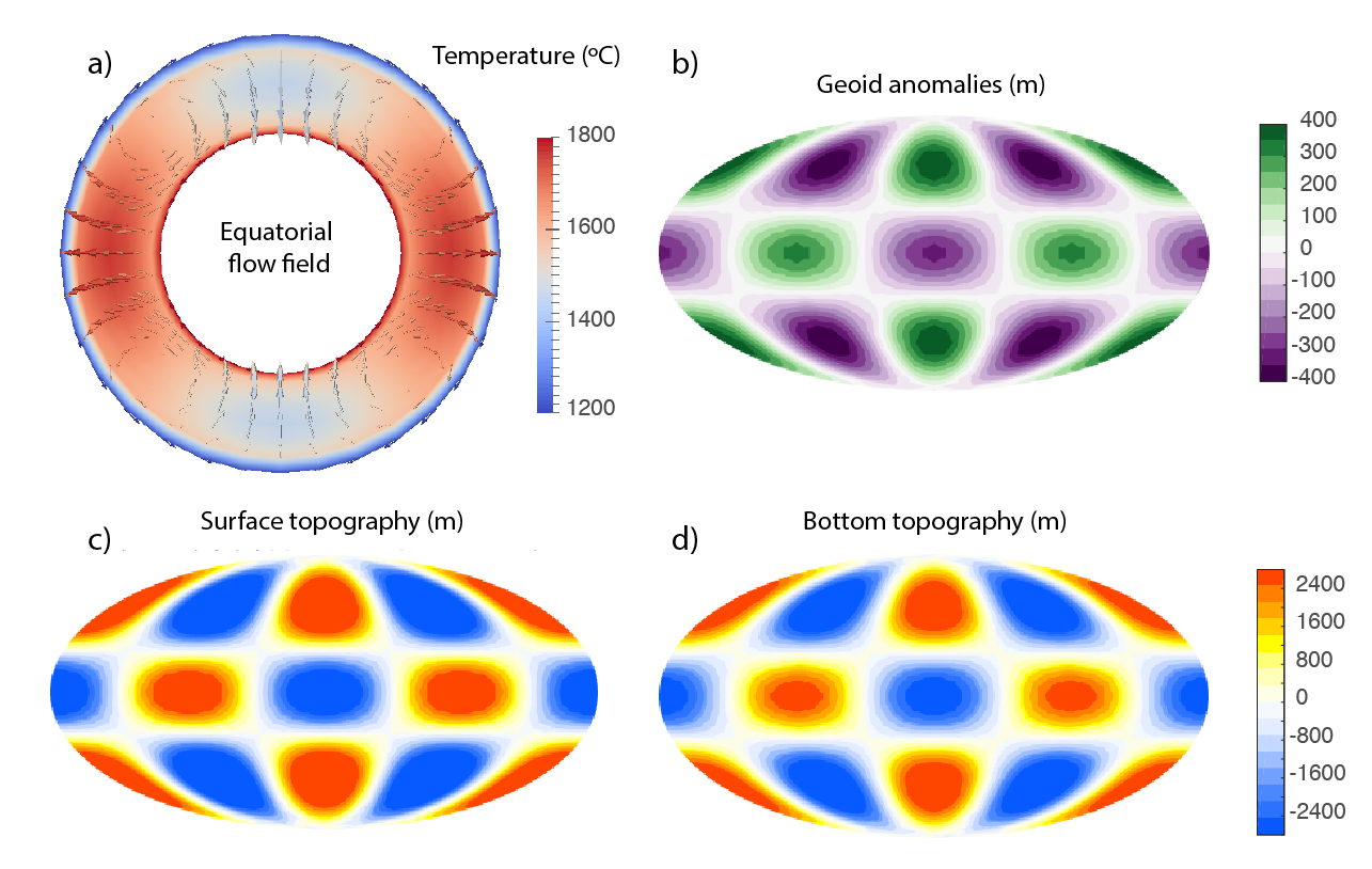
Fig. 84 Panel (a) shows an equatorial cross section of the temperature distribution and resulting flow from a harmonic perturbation. Panel (b) shows the resulting geoid, and panels (c) and (d) show the resulting surface and bottom topography. Note that we have subtracted the mean surface and bottom topography in the respective panels (c and d) as a postprocessing step outside of Aspect.