1D test for water solubility#
The implementation of the two-phase flow equations in ASPECT does not only describe the flow of a silicate melt through porous rocks, but can also be used to model the flow of other fluids, such as water. Water in the Earth’s mantle can either be bound in minerals, or it can be present as a fluid phase that can migrate relative to the solid rock. The fraction of this free water then represents the porosity of the material. Therefore, the terms describing melting and freezing of a silicate melt in the equations would instead describe the release and reabsorption of water (or other volatiles) into the rock, which are governed by the water (volatile) solubility.
This test shows how a model for water solubility can be implemented in a material model in ASPECT, and demonstrates the mass of water is conserved as water is released, migrates and is being reabsorbed. Specifically, in this test material with a water content of 1% flows into the model from the bottom. The model has three layers with different water solubility, specifically, and infinite solubility above 30 km depth and below 60 km depth, and a zero solubility in between. When the upwelling material reaches the boundary at 60 km depth, water is being released and can move relative to the solid as a free fluid phase. Due to its lower density, it moves upwards faster than the solid, until it reaches 30 km depth where it is reabsorbed into the solid. In steady state, the water content should be the same in the top and bottom layer, and in the middle layer it should be lower, proportional to the ratio between solid and melt velocity.
Specifically, the material properties are chosen in such a way that the free water moved twice as fast as the solid, so the porosity in the middle layer should be half of what flows in from the bottom, or 0.5%. This is illustrated in the visualizations below (Figure Fig. 209).
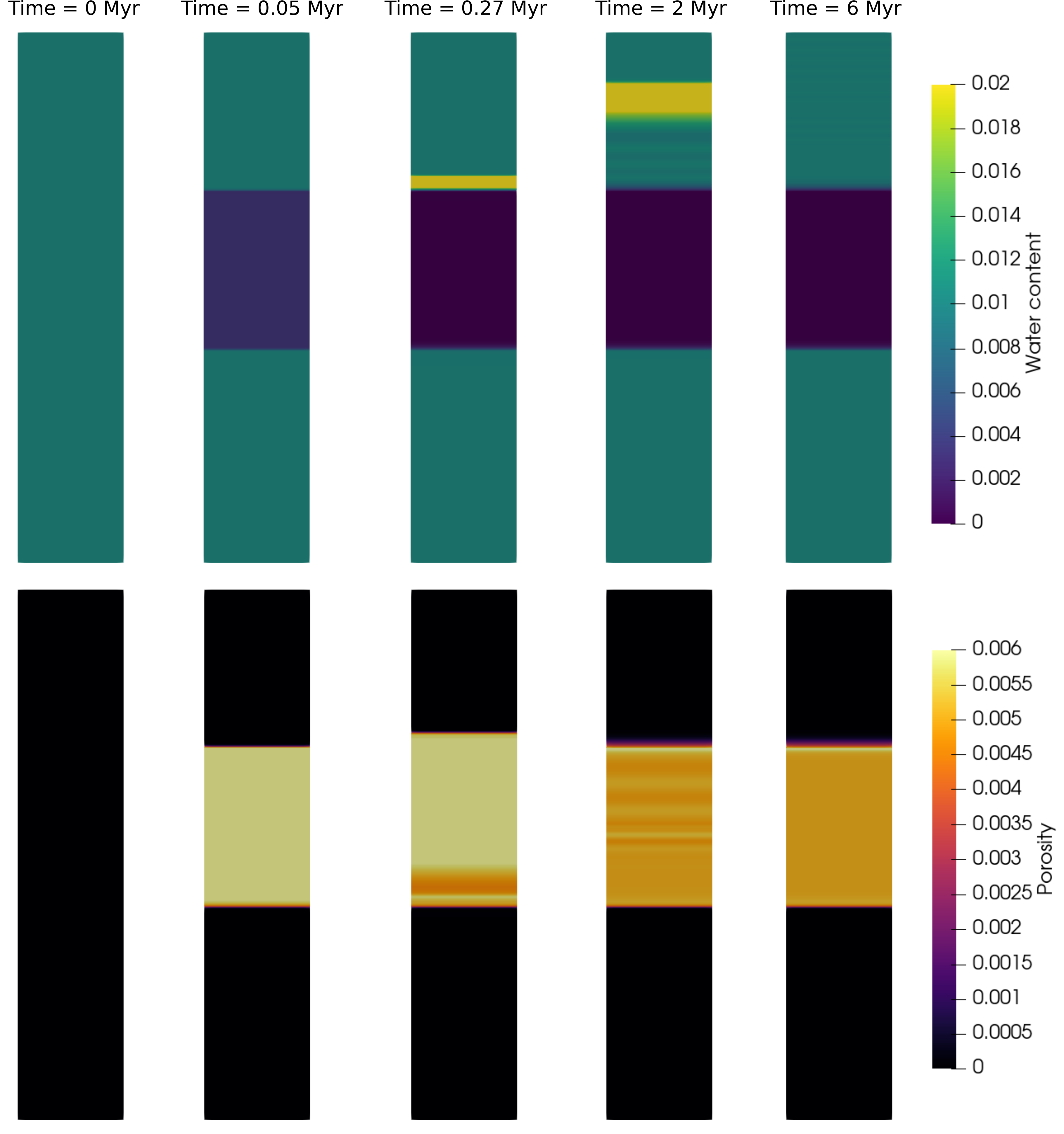
Fig. 209 Evolution of the bound water content (top) and the free water (bottom). Initially, all water is bound. Since the middle layer has a zero solubility, water is released and starts migrating upward with respect to the solid, initially leading to a higher bound water content when it reaches the top layer. As the model reaches steady state, the (bound) water content in the top and bottom layer are equal (1%) and the water content in the middle layer is 0.5%.#
Note that this example is specifically for water, but the general concept can be applied to a fluid of an arbitrary composition.
The benchmark can be run using the parameter files in benchmarks/solubility/. The material model is implemented in benchmarks/solubility/plugin/solubility.cc. Consequently, this code needs to be compiled into a shared library before you can run the test.
# This is a 1D test case for the solubility of fluids in interaction
# with porous flow. Material with a given water content flows into the
# model from the bottom. The model has three layers with different
# water solubility, specifically, an infinite solubility above 30 km
# depth and below 60 km depth, and a zero solubility in between. When
# the upwelling material reaches the boundary at 60 km depth, water is
# being released and can move relative to the solid as a free fluid
# phase. Due to its lower density, it moves upwards faster than the
# solid, until it reaches 30 km depth where it is reabsorbed into the
# solid. In steady state, the water content should be the same in the
# top and bottom layer, and in the middle layer it should be lower,
# proportional to the ratio between solid and melt velocity.

set Additional shared libraries            = ./plugin/libsolubility.so
set Adiabatic surface temperature          = 1600
set Nonlinear solver scheme                = iterated Advection and Stokes
set Output directory                       = output
set Max nonlinear iterations               = 10
set Nonlinear solver tolerance             = 1e-5

# The number of space dimensions you want to run this program in.
set Dimension                              = 2
set End time                               = 6e6

# Because the model includes reactions that might be on a faster time scale
# than the time step of the model (melting and the freezing of melt), we use
# the operator splitting scheme.
set Use operator splitting                     = true

subsection Solver parameters
  subsection Operator splitting parameters
    # We choose the size of the reaction time step as 200 years, small enough
    # so that it can accurately model melting and freezing.
    set Reaction time step                     = 1e4

    # Additionally, we always want to do at least 10 operator splitting time
    # steps in each model time step, to accurately compute the reactions.
    set Reaction time steps per advection step = 10
  end
end

# There are two compositional fields, one that tracks the amount of free water
# (the porosity) and one that tracks the amount of bound water (the water_content).
subsection Compositional fields
  set Number of fields = 2
  set Names of fields = porosity, water_content
end

# Initially, there is no free water (the porosity is zero) and the water content
# of the material is 1%.
subsection Initial composition model
  set Model name = function

  subsection Function
    set Function expression = 0.0; 0.01
  end
end

# The material flowing in from the bottom has the same water content as prescribed
# in the initial condition.
subsection Boundary composition model
  set Fixed composition boundary indicators   = bottom
  set List of model names = initial composition
end

# We prescribe an upwelling velocity of 1 cm/yr at the bottom,
# the left and right boundaries are closed and the top is open.
subsection Boundary velocity model
  set Tangential velocity boundary indicators = left, right
  set Prescribed velocity boundary indicators = bottom:function

  subsection Function
    set Function expression = 0; 1e-2
  end
end

# The model is 1 km wide and extends 100 km in vertical direction.
# This is because for this specific test material model, the transitions
# between the three layers with different water solubilities are at
# 30 km and 60 km depth.
subsection Geometry model
  set Model name = box

  subsection Box
    set X extent  = 2e2
    set Y extent  = 1e5
    set Y repetitions = 500
  end
end

subsection Gravity model
  set Model name = vertical

  subsection Vertical
    set Magnitude = 10.0
  end
end

# The temperature is not important for this model, so we simply
# set it to 1600 K everywhere (including the boundary).
subsection Initial temperature model
  set Model name = function

  subsection Function
    set Function expression = 1600
  end
end

subsection Boundary temperature model
  set Fixed temperature boundary indicators   = top, bottom
  set List of model names = initial temperature

  subsection Initial temperature
    set Maximal temperature = 1600
    set Minimal temperature = 1600
  end
end

# We use a custom material model that implements the layers with
# different solubility.
subsection Material model
  set Model name = volatiles

  subsection Volatile model
    set Base model = visco plastic
    set Reference fluid density = 2995
    set Shear to bulk viscosity ratio = 0.1
    set Reference fluid viscosity = 10
    set Reference permeability = 2.5e-6
    set Exponential fluid weakening factor = 27
    set Fluid reaction time scale for operator splitting = 5e4
  end

  subsection Visco Plastic
    set Reference temperature                   = 1600
    set Prefactors for diffusion creep          = 5e-21
    set Viscous flow law = diffusion
    set Densities                   = 3000
    set Viscosity averaging scheme  = harmonic
    set Minimum viscosity           = 1e19
    set Maximum viscosity           = 1e19
  end
end

subsection Mesh refinement
  set Coarsening fraction                      = 0.0
  set Refinement fraction                      = 0.0
  set Initial adaptive refinement              = 0
  set Initial global refinement                = 0
  set Strategy                                 = composition
  set Time steps between mesh refinement       = 0
end

subsection Melt settings
  set Include melt transport                  = true
end

subsection Postprocess
  set List of postprocessors = visualization, composition statistics, velocity statistics

  subsection Visualization
    set List of output variables      = density, viscosity, thermal expansivity, melt material properties, melt fraction
    set Output format                 = vtu
    set Time between graphical output = 0
    set Interpolate output            = false

    subsection Melt material properties
      set List of properties          = fluid density, permeability, fluid viscosity, compaction viscosity
    end
  end
end