Brittle thrust wedges benchmark

This section was contributed by Sibiao Liu, Stephanie Sparks, John Naliboff, Cedric Thieulot, and Wolfgang Bangerth.

Thrusting of brittle crust by applying compressive forces can lead to large deformations. The process is complicated to model because the rheology of cold, brittle crust is substantially more complicated than that of the hot, ductile rocks in the mantle. At the same time, the processes that act in such situations are surprisingly easy to replicate and visualize using simple “sand box” experiments in which one fills a volume with layers of differently-colored sand and compresses or stretches the volume. Examples of the patterns one can then observe in these do-it-yourself models are shown in Fig. 234 and Fig. 235.

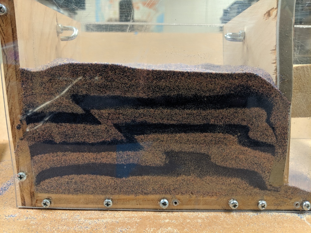
Fig. 234 Examples of deformation patterns of “sand box” experiments in which alternating layers of differently-colored sand undergo deformation. Pictures courtesy of the lab of Dennis Harry at Colorado State University.

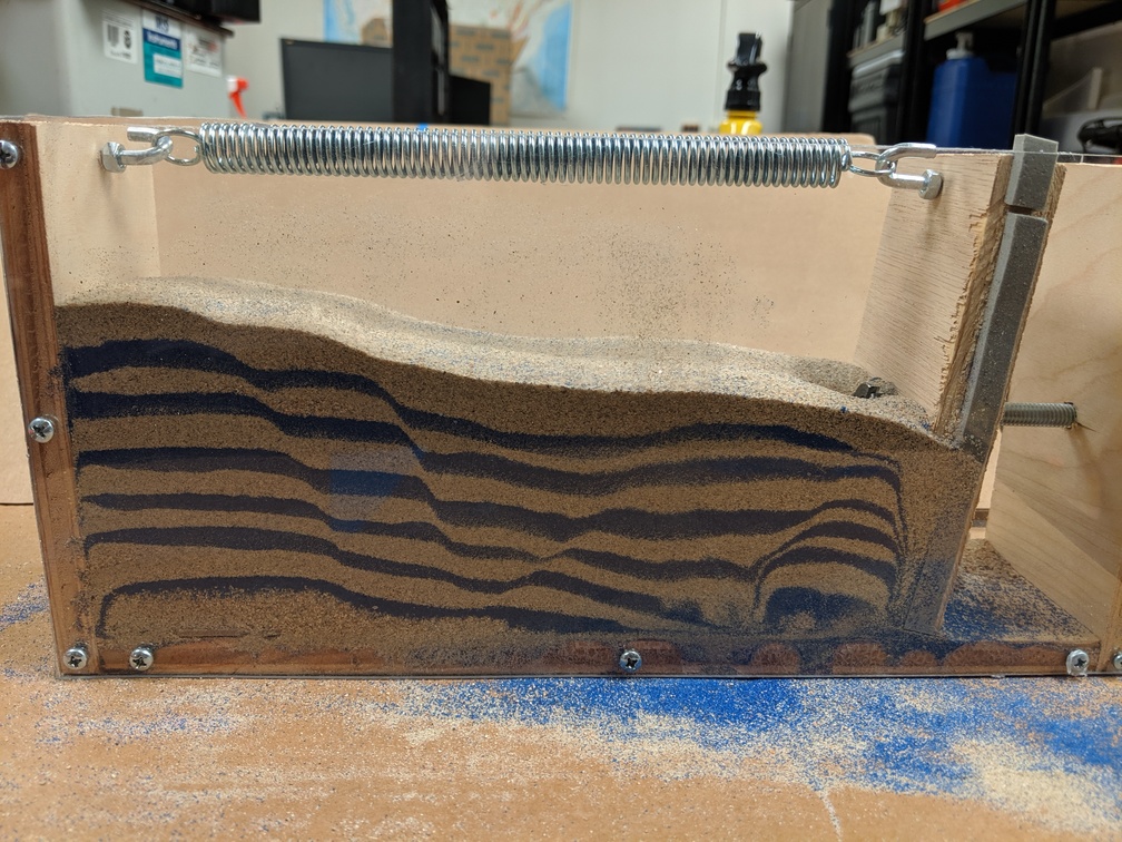
Fig. 235 Examples of deformation patterns of “sand box” experiments in which alternating layers of differently-colored sand undergo deformation. Pictures courtesy of the lab of Dennis Harry at Colorado State University.

[Buiter et al., 2016] organized new comparison experiments between these kinds of analogue and numerical models to investigate this kind of brittle thrust wedge behavior. The benchmark here aims to verify that the wedge models using follows other numerical results and the analytical wedge theory shown in this paper. In particular, input files (benchmarks/buiter_et_al_2016_jsg) are provided for reproducing the numerical simulations of stable wedge experiment 1 and unstable wedge experiment 2 with the same model setups.

A number of model sets of prescribed material behavior are required to simulate the brittle thrust formation. For example, although the material in the numerical model has a visco-plastic rheology, it performs plastic yielding at the beginning of shortening due to the non-viscous sand. We prescribe plastic strain-weakening behavior, with the internal angle of friction diminishing between total finite strain invariant values of 0.5 and 1.0, to mimic the softening from peak to dynamic stable strength which correlates with sand dilation.

In sandbox-type models, an important role is played by the boundaries and the frictional sliding of sand against these boundaries. For the top boundary condition, zero traction (“open”) and a sticky air layer is used to approximate a free surface. Additional testing revealed that using a true free surface leads to significant mesh distortion and associated numerical instabilities. We also apply a rigid block that approximates a mobile wall with a constant velocity of 2.5 cm/hour on the right-hand side boundary to drive the deformation in the sand layers. The following listing shows key portions of the parameter file that describes this kind of setup:

# Spatial domain of different compositional fields:
# Quartz sand (qsand) has two layers with 1 cm thickness each.
# Corundum sand (csand) is in the middle of the 2-layer quatz sand and is
# 1 cm thick.
# The boundary 2-mm-thin layers (bound) sit on both the bottom of the domain and
# between the sand and rigid indenter block. The right boundary has a constant
# inflow velocity, which pushes a rigid block that approximates a mobile wall.
# Movement of the rigid block drives deformation in the sand layers.
# The boundary between the rigid block and boundary layers produces a sharp
# velocity discontinuity that localizes brittle deformation.
# The sticky air layer is set on top of the sand layer and approximates a
# free surface.

# Velocity boundary conditions
subsection Boundary velocity model
  set Zero velocity boundary indicators              = bottom    #no slip
  set Tangential velocity boundary indicators        = left      #free slip

  # right - material inflow with a velocity of 2.5 cm/hour at the height of
  # the pushing block. The velocity linearly decreases from the base of the
  # rigid block to 0 cm/hour at the base of the model.
  set Prescribed velocity boundary indicators        = right:function

  subsection Function
    set Variable names                             = x,y
    set Function constants                         = cm=0.01, h=3600, th=0.002
    set Function expression                        = if(y>th, -2.5*cm/h, -(y/th)*2.5*cm/h); 0
  end
end

# The top boundary is open (zero traction), which allows the sticky air to
# flow freely through it as topography develops along the wedge. Additional
# testing revealed that using a true free surface leads to significant mesh
# distortion and associated numerical instabilities.
subsection Boundary traction model
  set Prescribed traction boundary indicators        = top: zero traction
end

Accurate solver convergence is always challenging to achieve in numerical thrust wedge models with a high spatial resolution (ca. 1 mm node spacing) and a large viscosity contrast. Here, we suggest that several parameters should be considered carefully. First, the nonlinear and linear solver tolerances should be sufficiently strict to avoid numerical instabilities. Second, we use the discontinuous Galerkin method (set Use discontinuous composition discretization = true) to ensure that the discontinuous composition bound preserving limiter produces sharp interfaces between compositional layers. Lastly, we use the harmonic averaging scheme for material and viscosity is required to achieve reasonable convergence behavior. The relevant parameters are shown here:

# Note that the Linear/Nonlinear solver tolerance should be sufficiently strict
# to avoid numerical instabilities.
set Nonlinear solver scheme                 = single Advection, iterated Stokes
set Nonlinear solver tolerance               = 1e-7
set Max nonlinear iterations                = 100

subsection Solver parameters
  subsection Stokes solver parameters
    set Linear solver tolerance             = 1e-8
    set Number of cheap Stokes solver steps = 0

    # A higher restart length makes the solver more robust for large viscosity
    # contrasts.
    set GMRES solver restart length         = 200
  end
end

# The  discontinuous composition bound preserving limiter produces sharp
# interfaces between compositional layers.
subsection Discretization
  set Use discontinuous composition discretization   = true

  subsection Stabilization parameters
    set Use limiter for discontinuous composition solution = true
    set Global composition maximum                 = 1, 1, 1, 1, 1, 100
    set Global composition minimum                 = 0, 0, 0, 0, 0, 0
  end
end

# Material properties
# Using harmonic material averaging is required to achieve reasonable
# convergence behavior, particulally when the viscosity contrast is large.
subsection Material model
  set Material averaging                             = harmonic average
  set Model name                                     = visco plastic

  subsection Visco Plastic
    # The viscosity contrast is 10^7 here and any value higher than this causes
    # divergence of the solver.
    set Minimum viscosity                            = 1e5
    set Maximum viscosity                            = 1e12
    set Viscosity averaging scheme                   = harmonic
  end
end

Experiment 1 tests whether model wedges in the stable domain of critical taper theory remain stable when translated horizontally. A quartz sand wedge with a horizontal base and a surface slope of 20 degrees is pushed 4 cm horizontally by inward movement of a mobile wall at the right boundary with a velocity of 2.5 cm/hour (Fig. 236). The basal angle is zero (horizontal), a thin layer separates the sand and boundary to ensure minimum coupling between the wedge and bounding box during translation, and a sticky air layer is used above the wedge. Further, the purely plastic material should not undergo any deformation during translation.

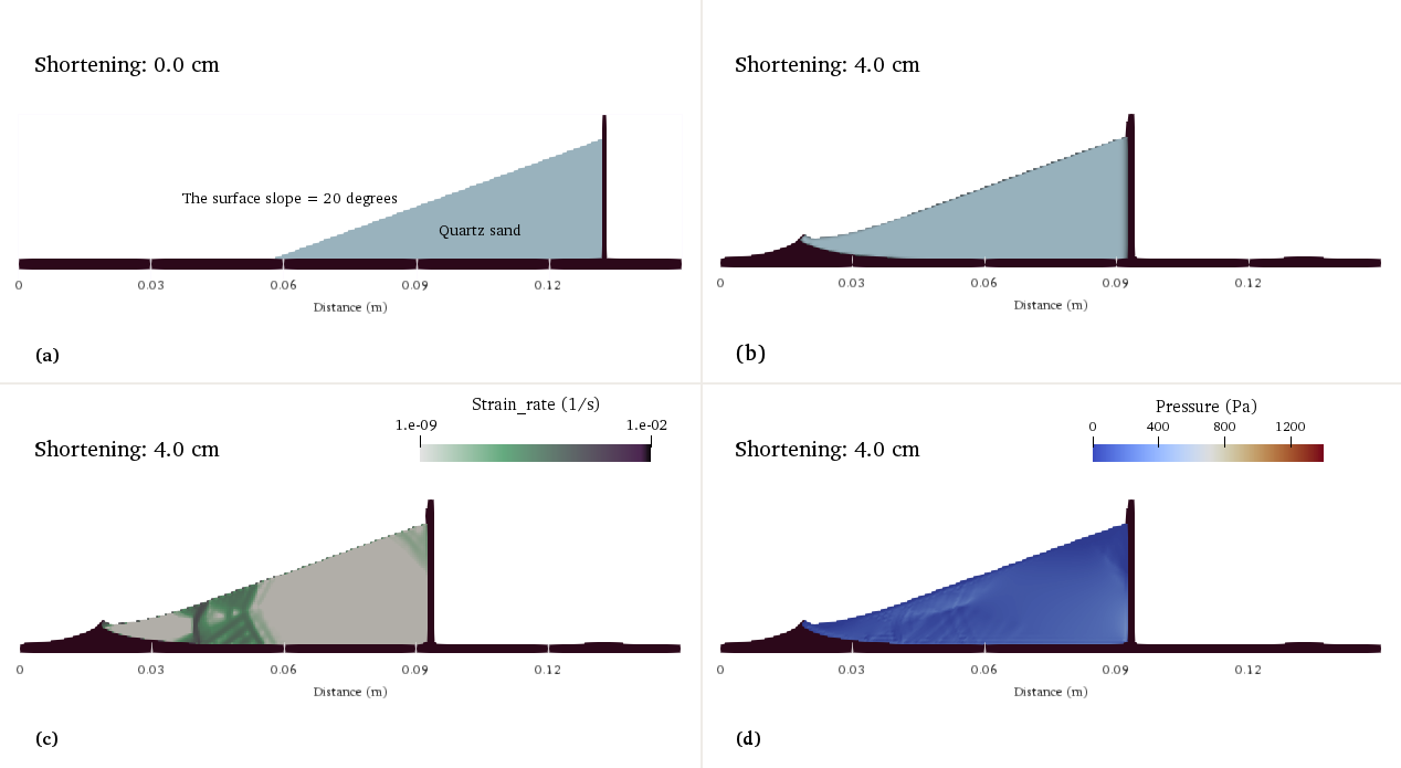
Fig. 236 Numerical model of a stable sand wedge. a) Initial model setup. b) Material field after 4 cm of translation. c) Strain rate field and d) pressure field.

Experiment 2 tests how an unstable subcritical wedge deforms to reach the critical taper solution. In this experiment, horizontal layers of sand undergo 10 cm shortening by inward movement of a mobile wall with a velocity of 2.5 cm/hour (Fig. 237). Model results show thrust wedge generation near the mobile wall through a combination of mainly in-sequence forward and backward thrusting. The strain field highlights several incipient shear zones that do not always accumulate enough offset to become visible in the material field. The pressure field of the model remains more or less lithostatic, with lower pressure values in (incipient) shear zones.

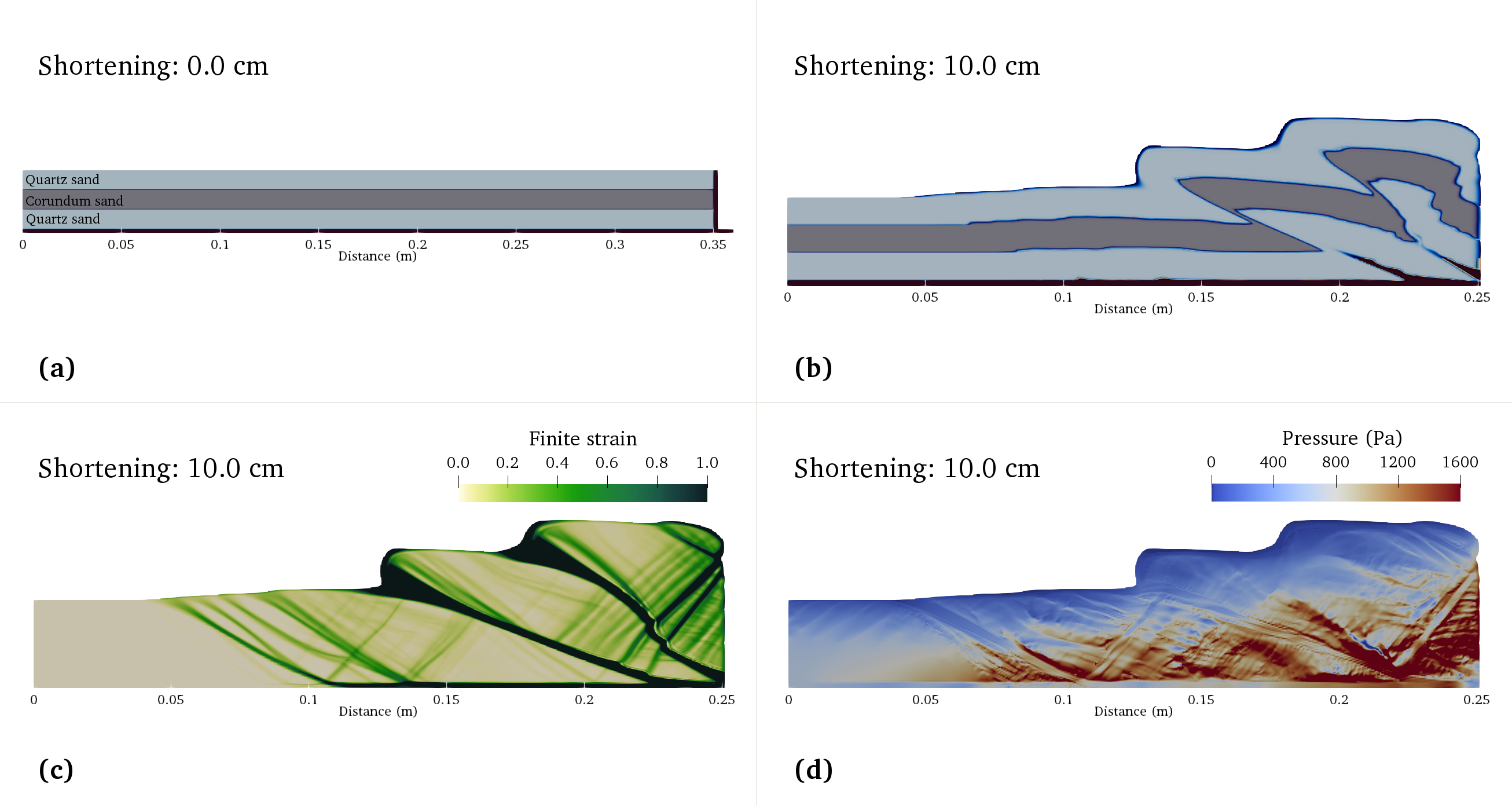
Fig. 237 Numerical model of an unstable subcritical wedge. a) Initial model setup. b) Material field of sands after 10 cm shortening. c) Strain field and d) pressure field.