Subduction initiation from Matsumoto and Tomoda (1983)#
This section was contributed by Cedric Thieulot.
The setup for this experiment originates in Matsumoto and Tomoda [1983].
In this very early computational geodynamics paper, the authors are interested in predicting the future process of crustal and lithospheric movement at the gigantic fracture zone in the Northeastern Pacific by means of numerical simulation of contact between two kinds of viscous fluid of different density. They then formulate the incompressible isothermal linear Stokes equations with a stream function approach and the resulting equation is solved by means of the Finite Difference method and the Marker and Cell (MAC) method.
The domain is a 2D Cartesian box of size \(L_x \times L_y=(400~\text{ km},180~\text{ km})\). There are three fluids in the domain: water (\(\rho_w=1030~\text{ kg m}^{-3}\), \(\eta_w=10^{-3}~\text{ Pa s}\)), lithosphere (\(\rho_l=3300~\text{ kg m}^{-3}\), \(\eta_l\)) and asthenosphere (\(\rho_a=3200~\text{ kg m}^{-3}\), \(\eta_a\)). Note that although the water viscosity is correct, this is probably not the value that was used by the authors since it would most likely lead to numerical errors. We thus set \(\eta_w=10^{19}~\text{ Pa s}\) (we can then speak of ‘sticky water’). Note that the choice of adequate viscosity for sticky air/water layers is discussed in depth in \cite{crameri:etal:2012}. Also, all viscosities in the paper are expressed in Poise with \(1~\text{ Poise}=0.1~\text{ Pa s}\).
The setup is shown in Fig. 131 and the list of simulations run by the authors is in Table 5.
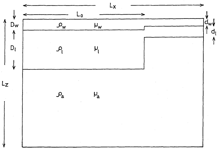
Fig. 131 \(D_w= 10~\text{ km}\), \(D_l= 50~\text{ km}\), \(d_w=8~\text{ km}\), \(d_l=10~\text{ km}\). These values represent the easternmost part of the Mendocino Fracture Zone. Taken from Matsumoto and Tomoda [1983].#
Case |
\(\eta_l~(\text{ Pa s})\) |
\(\eta_a~(\text{ Pa s})\) |
domain size (km) |
|---|---|---|---|
1 |
\(10^{22}\) |
\(10^{21}\) |
\(400\times 180\) |
2 |
\(10^{22}\) |
\(10^{20}\) |
\(400\times 180\) |
3 |
\(10^{22}\) |
\(10^{19}\) |
\(400\times 180\) |
4 |
\(10^{23}\) |
\(10^{21}\) |
\(400\times 180\) |
5 |
\(10^{22}\) |
\(10^{20}\) |
\(800\times 140\) |
6 |
\(10^{22}\) |
\(10^{19}\) |
\(800\times 140\) |
Rather interestingly the model is built in such a way that the lithostatic pressure is uniform at the bottom of the domain. Models are run for 50 Myr. Boundary conditions are free-slip on all sides of the domain. Unfortunately the authors do not specify the mesh resolution that was used but Fig. 132 gives us an idea.
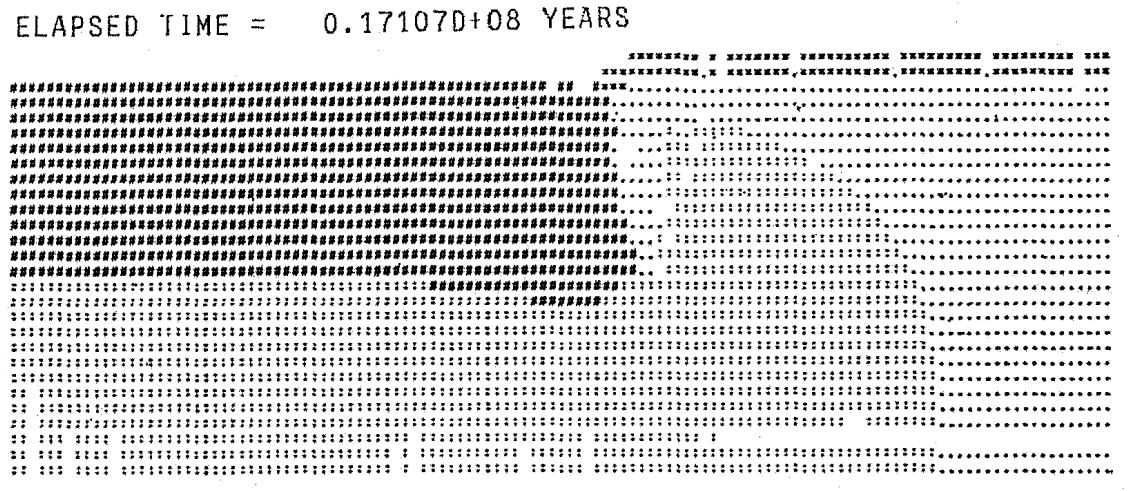
Fig. 132 Computer output of the result of Case 6(c). # indicates a particle representing the material of older lithosphere, * is that of younger lithosphere, : is older asthenosphere and \(\cdot\) is younger asthenosphere. Taken from Matsumoto and Tomoda [1983].#
Two parameter files are provided for Case 1: one using compositional fields, and one using the particle-in-cell approach. Other cases can be run by changing the viscosities and/or the domain size accordingly in the parameter files. Note that changing the domain size does not just require changing the geometry model, but also the initial composition model.
Results for Case 1 in the original publication are shown in Fig. 133 and results obtained in ASPECT are shown in Fig. 134.
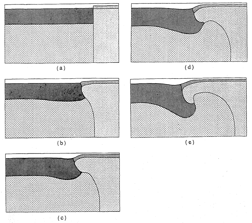
Fig. 133 Results of calculation in Case 1. (a) 0 Ma; (b) 12 Ma; (c) 21.4 Ma; (d) 30.7 Ma; (e) 46.7 Ma. Taken from Matsumoto and Tomoda [1983].#
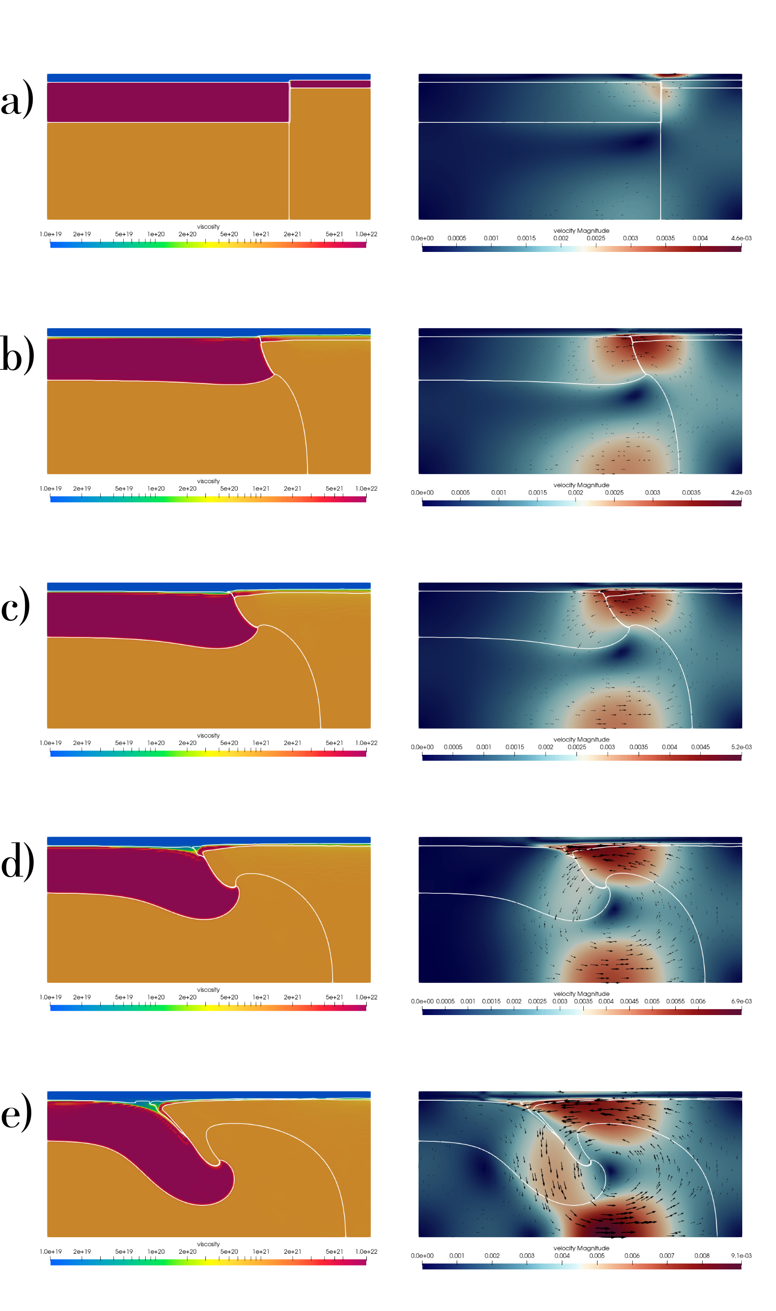
Fig. 134 Case 1 (obtained with the compositional fields approach) at (a) 0 Ma; (b) 12 Ma; (c) 21 Ma; (d) 31 Ma; (e) 41 Ma. Left column is density [kg/m\(^3\)], right column is velocity magnitude [m/year].#