Choosing a nonlinear Stokes solver#
When the problem to solve in ASPECT is nonlinear, choosing the right nonlinear solver scheme can be crucial to get fast convergence to the correct solution or even to converge at all. This section is aimed at explaining the differences between the three approaches available in ASPECT: iterated Stokes, iterated defect correction Stokes and Newton Stokes. The actual nonlinear Stokes solver you choose will also dictate which advection solver you choose, but we won’t discuss this choice in this section.
This section is structured as follows: first we will define the necessary terms by looking at a linear system and then the three solver options are explained very generically by looking at solving for \(\sin(x)=0\). Next, the options for the Newton solver will be explained, including how the stabilization works, and we end with the results of some simple test cases.
Solving a linear system#
When we try to solve a system of equations, we can write it down as:
where \(A\) is a known value or matrix, \(x\) is a unknown scalar or vector of unknowns, and \(b\) is the known right hand side scalar/vector. If we now want to know what \(x\) is for a given \(A\) and \(b\), we can rearrange the equation to:
where \(A^{-1}\) is the inverse of \(A\). In 1D a concrete example would be \(A=2\), \(b=5\), we would get:
Solving a nonlinear system#
Making the problem non-linear in our context means that \(A\) becomes dependent on \(x\). We can write this down as \(A(x)\). So our equation becomes:
To solve this nonlinear equation, we need to iterate. To illustrate this we are going to try to find \(x\) for \(\frac{1}{sqrt(1+x^2)}x = 0.5\). The function, the location of the solution and the location of the initial guess are shown in Fig. 2.
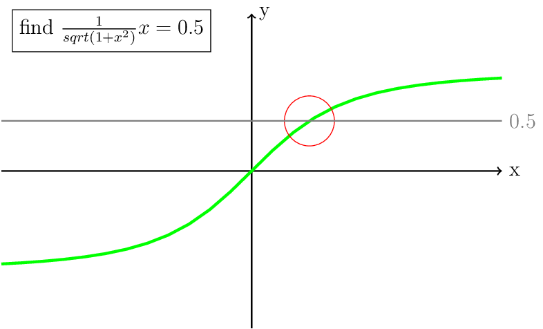
Fig. 2 The green line is the function \(\frac{1}{sqrt(1+x^2)}x = 0.5\), the gray line is at \(y = 0.5\) and the red circle indicates where the solution is going to be located.
As a basis for the next discussion, we will zoom in a bit on the known solution.
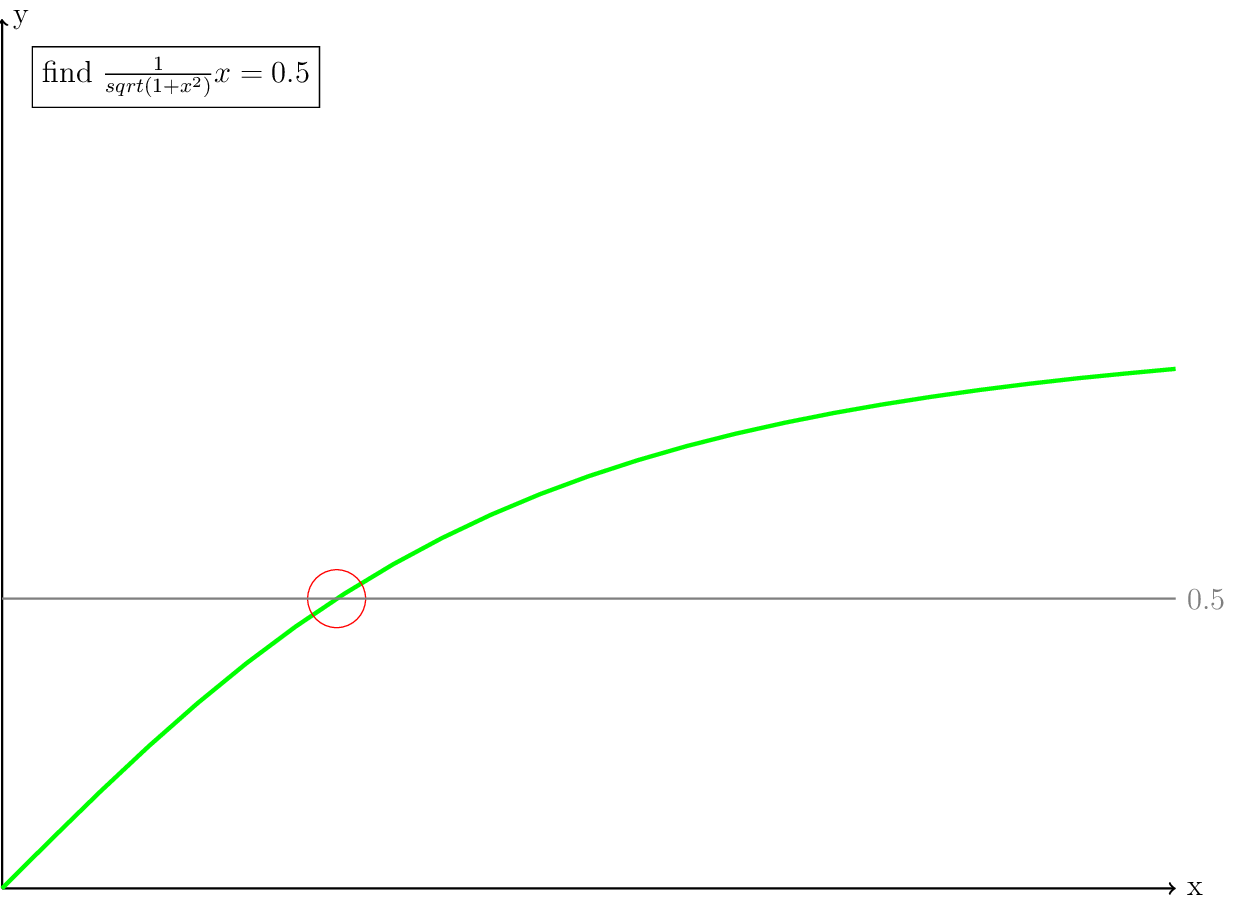
Fig. 3 Zoom of the previous figure.
Looking at the graph in Fig. 3, it is easy to see where the solution must be. Now imagine that you cannot see the whole graph at once, but you can only ask for the values of one \(x\) at a time. You could try every possible \(x\) value, but that would take a lot of attempts to get close to the solution. Another approach would be a bisect algorithm. A more robust way of solving the problem is called the Picard iteration, which we will discuss in the next section. An algorithm which converges much faster when it is close to the solution is the Newton iteration which we will discuss after the Picard iteration.
The full Picard iteration#
To solve this nonlinear equation using Picard iterations, we need to rewrite our equation in the form \(x = f(x)\). With the equation we have, this is actually quite easy:
This means that we need to find the point where \(x\) is equal to \(0.5*sqrt(1+x^2)\). The resulting \(x\) is a the same time the solution to our original question (see the gray lines in Fig. 4).
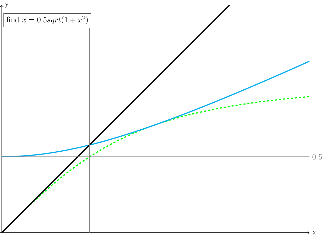
Fig. 4 A plot of the rewritten equation (cyan): \(x = 0.5*sqrt(1+x^2)\). The green line is the original equation, the black line is where x=y, and the gray lines intersect at the solution.
The Picard iteration transforms \(x = 0.5\cdot\sqrt{1+x^2}\) into \(x_{k+1} = 0.5 \cdot\sqrt{1+x_k^2}\). This means to start the iteration, we will need an initial guess where the solution is. Let’s pick \(x_0 = 2\).
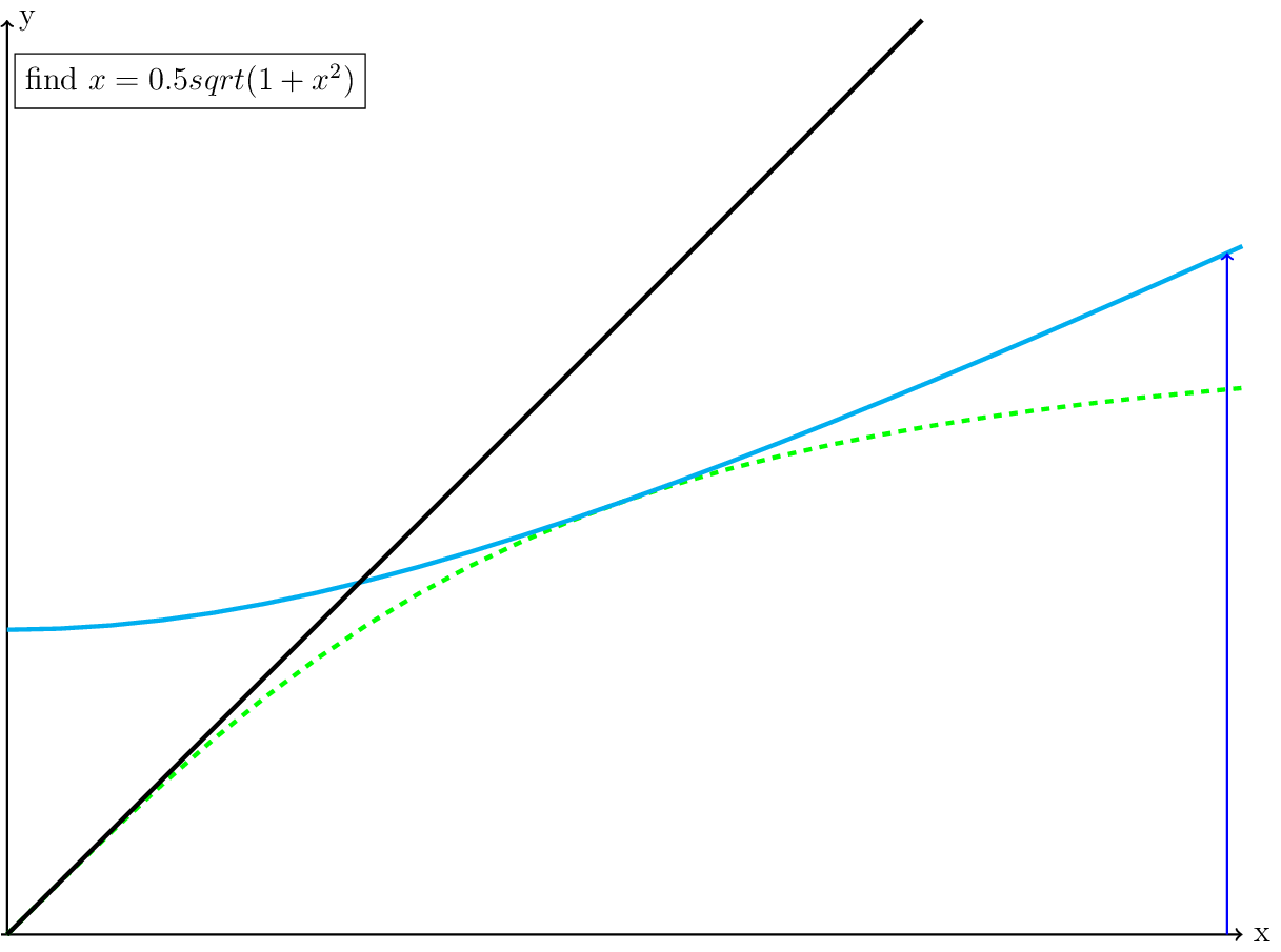
Fig. 5 The blue line is the location of our initial guess, \(x_0 = 2\).
Following the iteration, we set our next x (\(x_1\)) equal to our \(y = 0.5\cdot\sqrt{1+(2^2)} \approx 1.11803\)
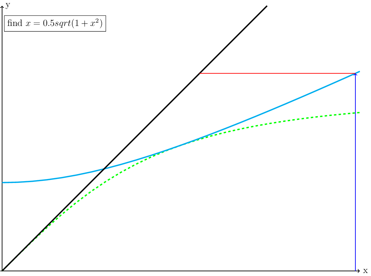
Fig. 6 The blue line is the location of our initial guess and the \(x=y\) step (red).
We then use the new \(x\) location to compute a new \(y\) and set \(x_2\) to that new \(y\). We keep repeating this until we are close enough to the solution:
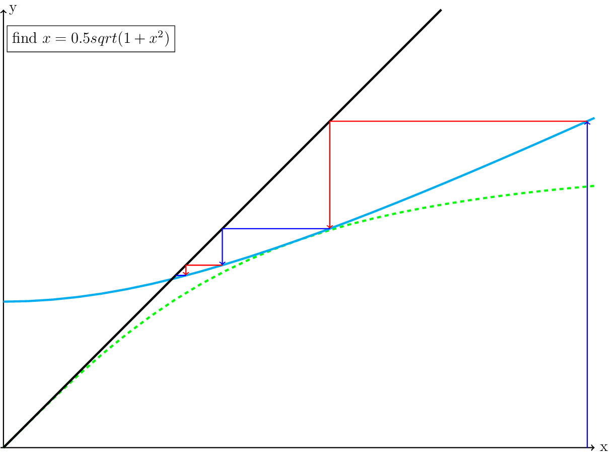
Fig. 7 Several Picard iterations colored blue and red for every other iteration.
Note that the closer the iteration gets to the solution, the slower the iteration converges. As shown in Fig. 4, the solution to this equation is the solution to the original equation. We can check that by substituting the \(x_{solution}\), which converges to \(\frac{1}{\sqrt{3}}\) into our original equation, and we get 0.5. In this case with the four iterations shown in Fig. 4, the final residual is \(0.5-\frac{1}{0.589624} \cdot 0.589624 = -0.00790859\).
In the context of ASPECT, the Picard iteration is usually written as
Because it looks very much like eq. (42), it is usually very easy to implement. It only requires a loop over the current linear solve feeding the current solution as the new guess.
Newton’s method#
Each Newton iteration can be written as \(x_{n+1} = x_n - \frac{f(x_n)}{f'(x_n)}\). This means that we are mostly interested in computing an update to the current solution. To compute the update we not only need to calculate \(f(x_n)\), but also the derivative \(f'(x_n)\). The iteration can be visualized in the same way as the Picard iteration but we won’t need the line \(x=y\) anymore. To better show some of the benefits and caveats of the Newton iteration, we will start with the equation \(\sin(x)=0\) and then go back to our current equation.
Solving \(\sin(x)=0\)#
We will start from a slightly different starting guess: \(x=1\). The derivative at \(x=1\) is \(\cos(1)\), so the new \(x_{n+1}\) becomes \(1-\frac{\sin(1)}{\cos(1)}=-0.557\).
There are a few things that are important to notice in Fig. 8. First, in practice each iteration can be represented as a vector with the origin at the solution of \((x,\sin(x))\) pointing in the direction of the derivative. This means that this vector has a certain length, which we will get back to later. Second, when the iteration converges, it can do so much faster than the Picard iteration. Third, when the initial guess is too far from the solution, the updated guess may be further away from the solution (Fig. 11). A special case of this is when the derivative is zero (Fig. 10). Both Fig. 10 and Fig. 11 visually show why it is important for the Newton iteration to have a good starting guess. Some strategies to achieve this, also called globalization, will be discussed in the section Globalization of the Newton iteration.
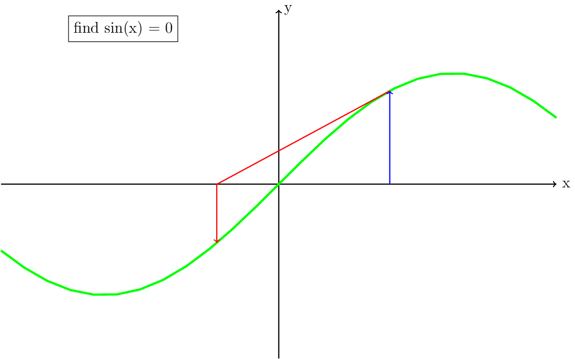
Fig. 8 Solving \(sin(x)=0\) through the Newton method with starting guess \(x=1\) and its derivative is plotted.
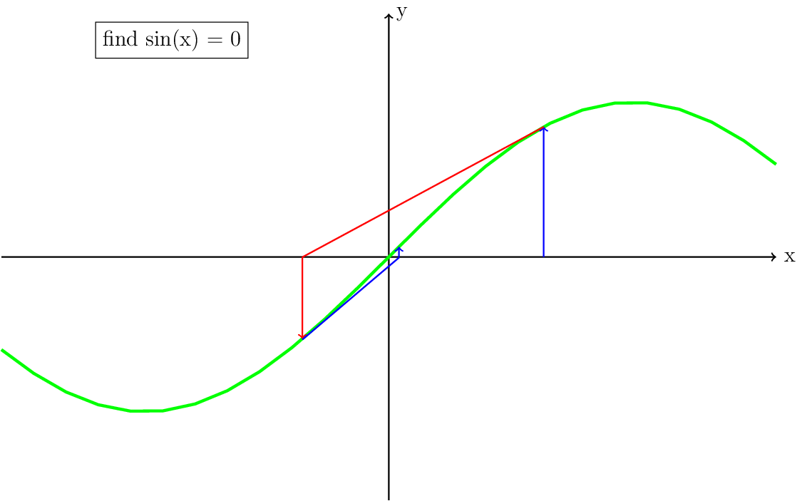
Fig. 9 Continuation from figure Fig. 8, with the blue lines showing one more iteration.
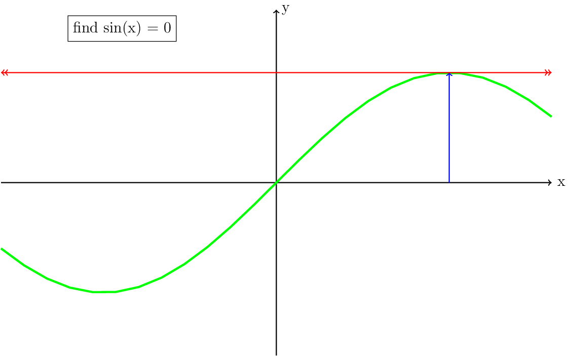
Fig. 10 Same as figure Fig. 8, but now showing the case where the initial guess leads to a derivative which is zero. This situation will cause a division by zero in the update and the solution will be undefined. For a system of equations, the linear solver will fail.
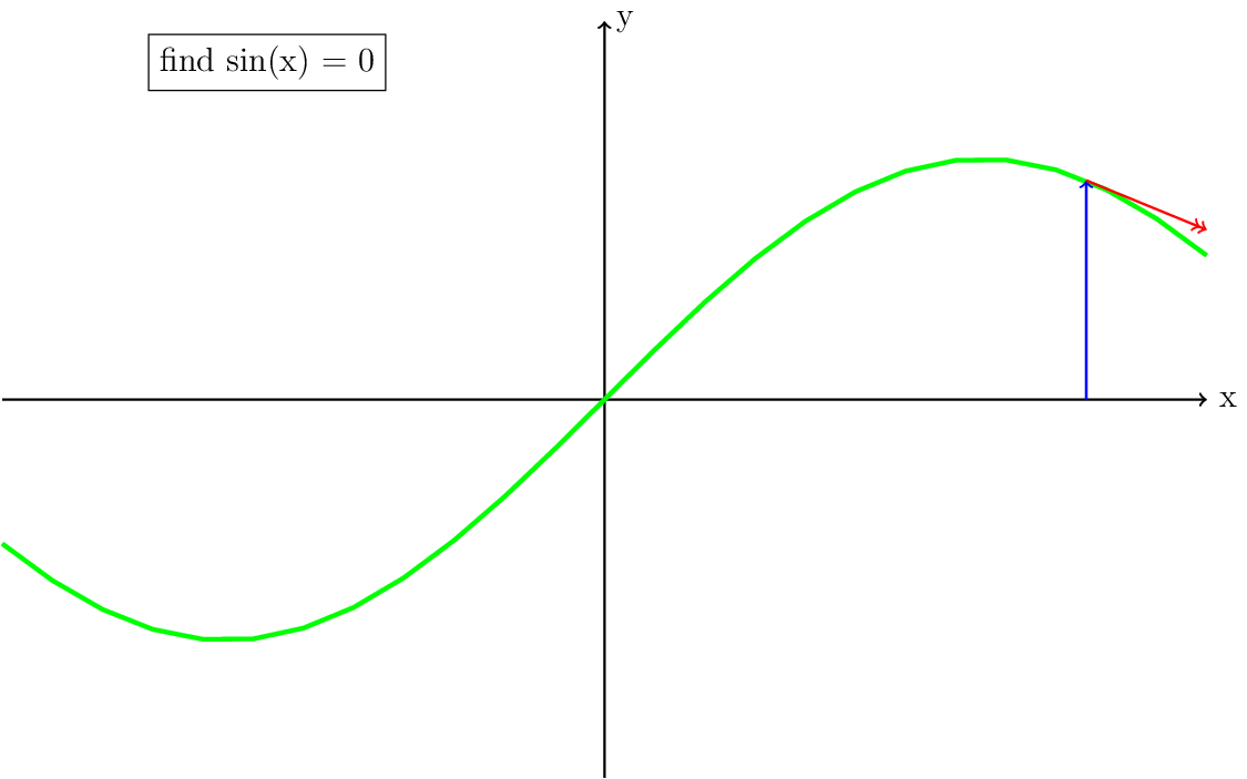
Fig. 11 Same as figure Fig. 8, but now showing the case where the initial guess is further away. In this case the direction of the next update will be further away from the solution and the iteration will diverge.
Solving \(\frac{1}{\sqrt{1+x^2}}x = 0.5\)#
Now that we have a general understanding of how the Newton solver works, let’s apply it to the equation we solved above with the Picard iteration. The method is going to be the same, but now we are stopping the derivative at the line \(y = 0.5\) instead of \(y = 0\). If we would take the initial guess at \(x=2\) the iteration would diverge, so we are taking the result from the first iteration of the Picard iteration, which is \(x = 1.11803\). This is a common tactic to achieve convergence in the Newton iteration and will be discussed further in the section Globalization of the Newton iteration.
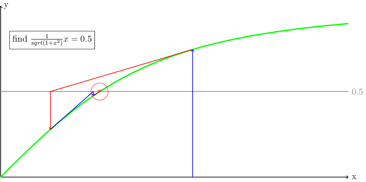
Fig. 12 The green line is the function \(\frac{1}{sqrt(1+x^2)}x = 0.5\), the gray line is at \(y = 0.5\) and the red circle indicates where the solution is going to be located.
The final residual after 3 Newton iterations, as shown in Fig. 12 is \(0.000567\) in three Newton iteration, starting from the result of the first Picard iteration. This means that with 1 Picard iteration and 3 Newton iterations, we got almost 14 times closer to the solution than with 4 Picard iterations.
Solving the Stokes equations in ASPECT#
For the Newton iteration, the equation is usually written as
In this equation, the right hand side (rhs) (\(A(x)x-b\) or \(-F\)) will be exactly zero when \(x\) is the exact solution to the nonlinear problem. Therefore, this is also called the residual. \(J\) is called the Jacobian, which is a derivative matrix for \(A\). In our simple example, this would just be the derivative. So we now solve for \(\delta x\) instead of \(x\):
Next we can compute the new solution with \(x_{n+1} = x_n - \delta x_n\). This form of computing an update/correction to the solution instead of computing the full solution every time is called a defect correction scheme.
For reasons beyond the scope of this section, depending on the rheology model, the Jacobian matrix may sometimes be the equivalent of figure Fig. 10, which means that the linear solver will fail. To stabilize this, there are some stabilization options available in ASPECT based on [Fraters et al., 2019], of which the most important is the SPD option. When you need to choose, it is important to know that the unstabilized version will always converge at the same speed or faster than the stabilized version. Theoretically this means that you will only want to stabilize when needed. This is an option for the Newton solver called the fail-safe. With the fail-safe you can run an unstabilized version of the Newton iteration, and when the linear solver fails, it will automatically turn on all the stabilizations for the rest of the timestep and retry the nonlinear iteration. The downside is that it may take a long time for the linear solver to fail, especially if it fails every timestep. So if you know that the model you are using is causing the linear solver to always fail, it is faster to just always turn on the stabilization. Note that the stabilization only works properly for the incompressible case.
Defect correction Picard iteration#
The last iteration scheme, the defect correction Picard iteration, is mathematically equivalent to the Picard iteration, but written in the form of the Newton solver. It turns out that the Jacobian in equation (43) internally consists of two parts:
If we approximate the Jacobian by setting it equal to \(A(x)\), the iteration will converge like a Picard iteration. The only difference is that computationally this defect correction form is more precise while requiring a less strict linear tolerance. This can speed up your computation and may help slightly with convergence in some cases.
Globalization of the Newton iteration#
Switch between the Picard and Newton iteration#
One of the easiest globalization strategies for the Newton solver is to first do a few Picard iterations. Remember that the Picard iteration will practically always converge (although for single iterations the residual may go up, the trend is usually down). Once you are close enough to the solution, switching to the Newton solver should then make the iteration converge quickly. The main issue is knowing when you are close enough to the solution so that the Newton solver works well. Unfortunately this threshold is problem dependent, but a combination between the different globalization options in this section should help.
Transition between the Picard and Newton iteration#
The change between the Picard and Newton iteration does not have to be a hard switch. When looking at equation (44), we can introduce a variable \(c_k\) and multiply it with \(A'(x)\):
When \(c_k\) is zero, the iteration behaves like a Picard iteration and when it is one, it behaves like a Newton iteration. In ASPECT we have implemented an option, which we refer to as the Residual Scaling Method (RSM). If enabled, this automatically computes \(c_k = \max\left(0.0,1.0-\frac{r_k}{r_{N_{DC}}}\right)\), where \(r_k\) is the current nonlinear residual and \(r_{N_{DC}}\) is the residual in the first iteration after switching to the Newton method. This option allows to more gradually switch to the Newton iteration and also gradually switch back if the iteration diverges.
Line search#
A Newton update can be seen as a hint in which direction to go with a suggestion for how much to go in that direction. But as we have seen, the size of the step can be much to big, which will lead the Newton iteration do diverge. The idea behind the line search is to use the direction, but check whether when applying the update to the solution, the residual has gotten smaller. If the residual has not gotten sufficiently smaller, then it scales this update step such that it is smaller until the next residual is sufficiently smaller than the current residual.
Some practical tips#
The Newton solver is a complex solver with many options, and without a bit of testing may actually be slower than using a Picard iteration. This may even be the case if it takes less iterations, since computing the derivatives for the Newton iteration can be expensive.
Always start with running a representative model with just a defect correction Picard iteration. Note that the defect correction Picard and the Newton method work well with much lower linear solver tolerances. A value of \(1e-2\) is a good default, but you may be able to even use \(1e-1\). If the nonlinear residual doesn’t converge quickly enough or at all to the desired nonlinear tolerance, then it is time to consider using the full Newton solver. It is strongly recommended to start by plotting the convergence behavior of the defect correction Picard method, with the number of nonlinear iterations on the x axis and the nonlinear residual on a logscale y axis. This will allow you to see the convergence behavior much more clearly than by just looking at the numbers in the ASPECT output file. Furthermore, it allows for a much better comparison with the convergence behavior of the Newton solver and between different settings of the Newton solver. For examples of such plots and more advice, please see section 3 of [Fraters et al., 2019].