Convection in a 2d box#

In this first example, let us consider a simple situation: a 2d box of dimensions $[0,1]\times [0,1]$ that is heated from below, insulated at the left and right, and cooled from the top. We will also consider the simplest model, the incompressible Boussinesq approximation with constant coefficients $\eta,\rho_0,\mathbf g,C_p, k$, for this testcase. Furthermore, we assume that the medium expands linearly with temperature. This leads to the following set of equations:

\[\begin{split}\begin{aligned} -\nabla \cdot \left[2\eta \varepsilon(\mathbf u) \right] + \nabla p &= \rho_0 (1-\alpha (T-T_0)) \mathbf g & \qquad & \textrm{in $\Omega$}, \\ \nabla \cdot \mathbf u &= 0 & \qquad & \textrm{in $\Omega$}, \\ \rho_0 C_p \left(\frac{\partial T}{\partial t} + \mathbf u\cdot\nabla T\right) - \nabla\cdot k\nabla T &= 0 & \qquad & \textrm{in $\Omega$}. \end{aligned}\end{split}\]

It is well known that we can non-dimensionalize this set of equations by introducing the Rayleigh number $Ra=\frac{\rho_0 g \alpha \Delta T h^3}{\eta \kappa}$, where $h$ is the height of the box, $\kappa = \frac{k}{\rho C_p}$ is the thermal diffusivity and $\Delta T$ is the temperature difference between top and bottom of the box. Formally, we can obtain the non-dimensionalized equations by using the above form and setting coefficients in the following way:

\[ \rho_0=C_p=\kappa=\alpha=\eta=h=\Delta T=1, \qquad T_0=0, \qquad g=Ra,\]

where $\mathbf g=-g \mathbf e_z$ is the gravity vector in negative $z$-direction. We will see all of these values again in the input file discussed below. One point to note is that for the Boussinesq approximation, as described above, the density in the temperature equation is chosen as the reference density $\rho_0$ rather than the full density $\rho(1-\alpha(T-T_0))$ as we see it in the buoyancy term on the right hand side of the momentum equation. As is able to handle different approximations of the equations (see Section Approximate equations), we also have to specify in the input file that we want to use the Boussinesq approximation. The problem is completed by stating the velocity boundary conditions: tangential flow along all four of the boundaries of the box.

This situation describes a well-known benchmark problem for which a lot is known and against which we can compare our results. For example, the following is well understood:

For values of the Rayleigh number less than a critical number $Ra_c\approx 780$, thermal diffusion dominates convective heat transport and any movement in the fluid is damped exponentially. If the Rayleigh number is moderately larger than this threshold then a stable convection pattern forms that transports heat from the bottom to the top boundaries. The simulations we will set up operates in this regime. Specifically, we will choose $Ra=10^4$.

On the other hand, if the Rayleigh number becomes even larger, a series of period doublings starts that makes the system become more and more unstable. We will investigate some of this behavior at the end of this section.
For certain values of the Rayleigh number, very accurate values for the heat flux through the bottom and top boundaries are available in the literature. For example, Blankenbach et al. report a non-dimensional heat flux of $4.884409 \pm 0.00001$, see Blankenbach et al. [1989]. We will compare our results against this value below.

With this said, let us consider how to represent this situation in practice.

The input file.#

The verbal description of this problem can be translated into an input file in the following way (see Parameter Documentation for a description of all of the parameters that appear in the following input file, and the indices at the end of this manual if you want to find a particular parameter; you can find the input file to run this cookbook example in cookbooks/convection-box.prm:

# A description of convection in a 2d box. See the manual for more information.


# At the top, we define the number of space dimensions we would like to
# work in:
set Dimension                              = 2

# There are several global variables that have to do with what
# time system we want to work in and what the end time is. We
# also designate an output directory.
set Use years in output instead of seconds = false
set End time                               = 0.5
set Output directory                       = output-convection-box

# Then there are variables that describe how the pressure should
# be normalized. Here, we choose a zero average pressure
# at the surface of the domain (for the current geometry, the
# surface is defined as the top boundary).
set Pressure normalization                 = surface
set Surface pressure                       = 0

# Then come a number of sections that deal with the setup
# of the problem to solve. The first one deals with the
# geometry of the domain within which we want to solve.
# The sections that follow all have the same basic setup
# where we select the name of a particular model (here,
# the box geometry) and then, in a further subsection,
# set the parameters that are specific to this particular
# model.
subsection Geometry model
  set Model name = box

  subsection Box
    set X extent = 1
    set Y extent = 1
  end
end

# The next section deals with the initial conditions for the
# temperature. Note that there are no initial conditions for the
# velocity variable since the velocity is assumed to always
# be in a static equilibrium with the temperature field.
# There are a number of models with the 'function' model
# a generic one that allows us to enter the actual initial
# conditions in the form of a formula that can contain
# constants. We choose a linear temperature profile that
# matches the boundary conditions defined below plus
# a small perturbation. The variables in this equation are
# described below, and it is important to note that in many
# cases the values correspond to other model parameters
# defined elsewhere. As such, if these model parameters are
# changed, the values below will also need to be adjusted.
#   L - Model length/width
#   p, k - values related to the small temperature perturbation

subsection Initial temperature model
  set Model name = function

  subsection Function
    set Variable names      = x,z
    set Function constants  = p=0.01, L=1, pi=3.1415926536, k=1
    set Function expression = (1.0-z) - p*cos(k*pi*x/L)*sin(pi*z)
  end
end

# Then follows a section that describes the boundary conditions
# for the temperature. The model we choose is called 'box' and
# allows to set a constant temperature on each of the four sides
# of the box geometry. In our case, we choose something that is
# heated from below and cooled from above, whereas all other
# parts of the boundary are insulated (i.e., no heat flux through
# these boundaries; this is also often used to specify symmetry
# boundaries).
subsection Boundary temperature model
  set Fixed temperature boundary indicators = bottom, top
  set List of model names = box

  subsection Box
    set Bottom temperature = 1
    set Left temperature   = 0
    set Right temperature  = 0
    set Top temperature    = 0
  end
end

# The next parameters then describe on which parts of the
# boundary we prescribe a zero or nonzero velocity and
# on which parts the flow is allowed to be tangential.
# Here, all four sides of the box allow tangential
# unrestricted flow but with a zero normal component:
subsection Boundary velocity model
  set Tangential velocity boundary indicators = left, right, bottom, top
end

# The following two sections describe first the
# direction (vertical) and magnitude of gravity and the
# material model (i.e., density, viscosity, etc). We have
# discussed the settings used here in the introduction to
# this cookbook in the manual already.
subsection Gravity model
  set Model name = vertical

  subsection Vertical
    set Magnitude = 1e4   # = Ra
  end
end

subsection Material model
  set Model name = simple

  subsection Simple model
    set Reference density             = 1
    set Reference specific heat       = 1
    set Reference temperature         = 0
    set Thermal conductivity          = 1
    set Thermal expansion coefficient = 1
    set Viscosity                     = 1
  end
end

# We also have to specify that we want to use the Boussinesq
# approximation (assuming the density in the temperature
# equation to be constant, and incompressibility).
subsection Formulation
  set Formulation = Boussinesq approximation
end

# The settings above all pertain to the description of the
# continuous partial differential equations we want to solve.
# The following section deals with the discretization of
# this problem, namely the kind of mesh we want to compute
# on. We here use a globally refined mesh without
# adaptive mesh refinement.
subsection Mesh refinement
  set Initial global refinement                = 4
  set Initial adaptive refinement              = 0
  set Time steps between mesh refinement       = 0
end

# The final part is to specify what ASPECT should do with the
# solution once computed at the end of every time step. The
# process of evaluating the solution is called `postprocessing'
# and we choose to compute velocity and temperature statistics,
# statistics about the heat flux through the boundaries of the
# domain, and to generate graphical output files for later
# visualization. These output files are created every time
# a time step crosses time points separated by 0.01. Given
# our start time (zero) and final time (0.5) this means that
# we will obtain 50 output files.
subsection Postprocess
  set List of postprocessors = velocity statistics, temperature statistics, heat flux statistics, visualization

  subsection Visualization
    set Time between graphical output = 0.01
  end
end

subsection Solver parameters
  set Temperature solver tolerance = 1e-10
end

Running the program.#

When you run this program for the first time, you are probably still running in debug mode (see Section Debug or optimized mode) and you will get output like the following:

Number of active cells: 256 (on 5 levels)
Number of degrees of freedom: 3,556 (2,178+289+1,089)

*** Timestep 0:  t=0 seconds
   Solving temperature system... 0 iterations.
   Rebuilding Stokes preconditioner...
   Solving Stokes system... 31+0 iterations.

[... ...]

*** Timestep 1085:  t=0.5 seconds
   Solving temperature system... 0 iterations.
   Solving Stokes system... 5 iterations.

   Postprocessing:
     RMS, max velocity:                  43.5 m/s, 70.3 m/s
     Temperature min/avg/max:            0 K, 0.5 K, 1 K
     Heat fluxes through boundary parts: 0.01977 W, -0.01977 W, -4.787 W, 4.787 W

Termination requested by criterion: end time


+---------------------------------------------+------------+------------+
| Total wallclock time elapsed since start    |      66.5s |            |
|                                             |            |            |
| Section                         | no. calls |  wall time | % of total |
+---------------------------------+-----------+------------+------------+
| Assemble Stokes system          |      1086 |      8.63s |        13% |
| Assemble temperature system     |      1086 |        32s |        48% |
| Build Stokes preconditioner     |         1 |    0.0225s |         0% |
| Build temperature preconditioner|      1086 |      1.52s |       2.3% |
| Solve Stokes system             |      1086 |       7.7s |        12% |
| Solve temperature system        |      1086 |     0.729s |       1.1% |
| Initialization                  |         1 |    0.0316s |         0% |
| Postprocessing                  |      1086 |      7.76s |        12% |
| Setup dof systems               |         1 |    0.0104s |         0% |
| Setup initial conditions        |         1 |   0.00621s |         0% |
+---------------------------------+-----------+------------+------------+

If you’ve read up on the difference between debug and optimized mode (and you should before you switch!) then consider disabling debug mode. If you run the program again, every number should look exactly the same (and it does, in fact, as I am writing this) except for the timing information printed every hundred time steps and at the end of the program:

+---------------------------------------------+------------+------------+
| Total wallclock time elapsed since start    |      25.8s |            |
|                                             |            |            |
| Section                         | no. calls |  wall time | % of total |
+---------------------------------+-----------+------------+------------+
| Assemble Stokes system          |      1086 |      2.51s |       9.7% |
| Assemble temperature system     |      1086 |      9.88s |        38% |
| Build Stokes preconditioner     |         1 |    0.0271s |      0.11% |
| Build temperature preconditioner|      1086 |      1.58s |       6.1% |
| Solve Stokes system             |      1086 |      6.38s |        25% |
| Solve temperature system        |      1086 |     0.542s |       2.1% |
| Initialization                  |         1 |     0.219s |      0.85% |
| Postprocessing                  |      1086 |      2.79s |        11% |
| Setup dof systems               |         1 |      0.23s |      0.89% |
| Setup initial conditions        |         1 |     0.107s |      0.41% |
+---------------------------------+-----------+------------+------------+

In other words, the program ran more than 2 times faster than before. Not all operations became faster to the same degree: assembly, for example, is an area that traverses a lot of code both in and out and so encounters a lot of verification code in debug mode. On the other hand, solving linear systems primarily requires lots of matrix vector operations. Overall, the fact that in this example, assembling linear systems and preconditioners takes so much time compared to actually solving them is primarily a reflection of how simple the problem is that we solve in this example. This can also be seen in the fact that the number of iterations necessary to solve the Stokes and temperature equations is so low. For more complex problems with non-constant coefficients such as the viscosity, as well as in 3d, we have to spend much more work solving linear systems whereas the effort to assemble linear systems remains the same.

Visualizing results.#

Having run the program, we now want to visualize the numerical results we got. ASPECT can generate graphical output in formats understood by pretty much any visualization program (see the parameters described in Section Subsection: Postprocess / Visualization) but we will here follow the discussion in Visualizing results and use the default VTU output format to visualize using the Visit program.

In the parameter file we have specified that graphical output should be generated every 0.01 time units. Looking through these output files (which can be found in the folder output-convection-box, as specified in the input file), we find that the flow and temperature fields quickly converge to a stationary state. Fig. 18 shows the initial and final states of this simulation.

../../../../../_images/convection_box_fields.svg — Fig. 18 Convection in a box: Initial temperature and velocity field (left) and final state (right).#

There are many other things we can learn from the output files generated by , specifically from the statistics file that contains information collected at every time step and that has been discussed in Visualizing statistical data. In particular, in our input file, we have selected that we would like to compute velocity, temperature, and heat flux statistics. These statistics, among others, are listed in the statistics file whose head looks like this for the current input file:

# 1: Time step number
# 2: Time (seconds)
# 3: Time step size (seconds)
# 4: Number of mesh cells
# 5: Number of Stokes degrees of freedom
# 6: Number of temperature degrees of freedom
# 7: Iterations for temperature solver
# 8: Iterations for Stokes solver
# 9: Velocity iterations in Stokes preconditioner
# 10: Schur complement iterations in Stokes preconditioner
# 11: RMS velocity (m/s)
# 12: Max. velocity (m/s)
# 13: Minimal temperature (K)
# 14: Average temperature (K)
# 15: Maximal temperature (K)
# 16: Average nondimensional temperature (K)
# 17: Outward heat flux through boundary with indicator 0 ("left") (W)
# 18: Outward heat flux through boundary with indicator 1 ("right") (W)
# 19: Outward heat flux through boundary with indicator 2 ("bottom") (W)
# 20: Outward heat flux through boundary with indicator 3 ("top") (W)
# 21: Visualization file name
... lots of numbers arranged in columns ...

Fig. 19 shows the results of visualizing the data that can be found in columns 2 (the time) plotted against columns 11 and 12 (root mean square and maximal velocities). Plots of this kind can be generated with Gnuplot by typing (see Visualizing statistical data for a more thorough discussion):

  plot "output-convection-box/statistics" using 2:11 with lines

Fig. [4][] shows clearly that the simulation enters a steady state after about $t\approx 0.1$ and then changes very little. This can also be observed using the graphical output files from which we have generated Fig.Convection in a box: Initial temperature and velocity field (left) and final state (right).. One can look further into this data to find that the flux through the top and bottom boundaries is not exactly the same (up to the obvious difference in sign, given that at the bottom boundary heat flows into the domain and at the top boundary out of it) at the beginning of the simulation until the fluid has attained its equilibrium. However, after $t\approx 0.2$, the fluxes differ by only $5\times 10^{-5}$, i.e., by less than 0.001% of their magnitude.[1] The flux we get at the last time step, 4.787, is less than 2% away from the value reported in (Blankenbach et al. 1989) ($\approx$4.88) although we compute on a $16\times 16$ mesh and the values reported by Blankenbach are extrapolated from meshes of size up to $72\times 72$. This shows the accuracy that can be obtained using a higher order finite element. Secondly, the fluxes through the left and right boundary are not exactly zero but small. Of course, we have prescribed boundary conditions of the form $\frac{\partial T}{\partial \mathbf n}=0$ along these boundaries, but this is subject to discretization errors. It is easy to verify that the heat flux through these two boundaries disappears as we refine the mesh further.

../../../../../_images/convection_box_stats.svg — Fig. 19 Convection in a box: Root mean square and maximal velocity as a function of simulation time (left). Heat flux through the four boundaries of the box (right).#

Furthermore, ASPECT automatically also collects statistics about many of its internal workings. Fig. 20 shows the number of iterations required to solve the Stokes and temperature linear systems in each time step. It is easy to see that these are more difficult to solve in the beginning when the solution still changes significant from time step to time step. However, after some time, the solution remains mostly the same and solvers then only need 9 or 10 iterations for the temperature equation and 4 or 5 iterations for the Stokes equations because the starting guess for the linear solver – the previous time step’s solution – is already pretty good. If you look at any of the more complex cookbooks, you will find that one needs many more iterations to solve these equations.

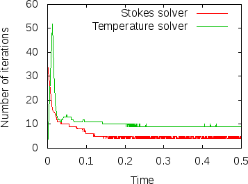
../../../../../_images/iterations.png — Fig. 20 Convection in a box: Number of linear iterations required to solve the Stokes and temperature equations in each time step.}#

Play time 1: Different Rayleigh numbers.#

After showing you results for the input file as it can be found in [cookbooks/convection-box.prm] (https://github.com/geodynamics/aspect/blob/main/cookbooks/convection-box/convection-box.prm), let us end this section with a few ideas on how to play with it and what to explore. The first direction one could take this example is certainly to consider different Rayleigh numbers. As mentioned above, for the value $Ra=10^4$ for which the results above have been produced, one gets a stable convection pattern. On the other hand, for values $Ra<Ra_c\approx 780$, any movement of the fluid dies down exponentially and we end up with a situation where the fluid doesn’t move and heat is transported from the bottom to the top only through heat conduction. This can be explained by considering that the Rayleigh number in a box is defined as $Ra=\frac{\rho_0 g\alpha\Delta T h^3}{\eta k}$. A small Rayleigh number below $Ra_c$ means that the buoyancy forces caused by temperature variations – $\rho_0 \alpha \Delta T$ – are not strong enough to overcome friction forces within the fluid, that is, the viscosity is too high.

On the other hand, if the Rayleigh number is large (i.e., the viscosity is small or the buoyancy large) then the fluid develops an unsteady convection period. As we consider fluids with larger and larger $Ra$, this pattern goes through a sequence of period-doubling events until flow finally becomes chaotic. The structures of the flow pattern also become smaller and smaller.

../../../../../_images/convection_box_fields_different_Ra.svg — Fig. 21 Convection in a box: Temperature fields at the end of a simulation for $Ra=10^2$ where thermal diffusion dominates (left) and Ra=10^6 where convective heat transport dominates (right). The mesh on the right is clearly too coarse to resolve the structure of the solution.#

../../../../../_images/convection_box_stats_different_Ra.svg — Fig. 22 Convection in a box: Velocities (left) and heat flux across the top and bottom boundaries (right) as a function of time at $Ra=10^6$.#

We illustrate these situations in Fig. 21 and Fig. 22. The first shows the temperature field at the end of a simulation for $Ra=10^2$ (below $Ra_c$) and at $Ra=10^6$. Obviously, for the right picture, the mesh is not fine enough to accurately resolve the features of the flow field and we would have to refine it more. The second of the figures shows the velocity and heatflux statistics for the computation with $Ra=10^6$; it is obvious here that the flow no longer settles into a steady state but has a periodic behavior. This can also be seen by looking at movies of the solution.

To generate these results, remember that we have chosen $g=Ra$ in our input file. In other words, changing the input file to contain the parameter setting

subsection Gravity model
  subsection Vertical
    set Magnitude = 1e6   # = Ra
  end
end

will achieve the desired effect of computing with $Ra=10^6$.

Play time 2: Thinking about finer meshes.#

In our computations for $Ra=10^4$ we used a $16\times 16$ mesh and obtained a value for the heat flux that differed from the generally accepted value from Blankenbach et al. (Blankenbach et al. 1989) by less than 2%. However, it may be interesting to think about computing even more accurately. This is easily done by using a finer mesh, for example. In the parameter file above, we have chosen the mesh setting as follows:

subsection Mesh refinement
  set Initial global refinement                = 4
  set Initial adaptive refinement              = 0
  set Time steps between mesh refinement       = 0
end

We start out with a box geometry consisting of a single cell that is refined four times. Each time we split each cell into its 4 children, obtaining the $16\times 16$ mesh already mentioned. The other settings indicate that we do not want to refine the mesh adaptively at all in the first time step, and a setting of zero for the last parameter means that we also never want to adapt the mesh again at a later time. Let us stick with the never-changing, globally refined mesh for now (we will come back to adaptive mesh refinement again at a later time) and only vary the initial global refinement. In particular, we could choose the parameter Initial global refinement to be 5, 6, or even larger. This will get us closer to the exact solution albeit at the expense of a significantly increased computational time.

A better strategy is to realize that for $Ra=10^4$, the flow enters a steady state after settling in during the first part of the simulation (see, for example, the graphs in Fig. 19). Since we are not particularly interested in this initial transient process, there is really no reason to spend CPU time using a fine mesh and correspondingly small time steps during this part of the simulation (remember that each refinement results in four times as many cells in 2d and a time step half as long, making reaching a particular time at least 8 times as expensive, assuming that all solvers in scale perfectly with the number of cells). Rather, we can use a parameter in the input file that let’s us increase the mesh resolution at later times. To this end, let us use the following snippet for the input file:

subsection Mesh refinement
  set Initial global refinement                = 3
  set Initial adaptive refinement              = 0
  set Time steps between mesh refinement       = 0
  set Additional refinement times              = 0.2, 0.3, 0.4
  set Refinement fraction                      = 1.0
  set Coarsening fraction                      = 0.0
end

What this does is the following: We start with an $8\times 8$ mesh (3 times globally refined) but then at times $t=0.2,0.3$ and $0.4$ we refine the mesh using the default refinement indicator (which one this is is not important because of the next statement). Each time, we refine, we refine a fraction 1.0 of the cells, i.e., all cells and we coarsen a fraction of 0.0 of the cells, i.e. no cells at all. In effect, at these additional refinement times, we do another global refinement, bringing us to refinement levels 4, 5 and finally 6.

../../../../../_images/convection_box_stats_steps.svg — Fig. 23 Convection in a box: Refinement in stages. Total number of unknowns in each time step, including all velocity, pressure and temperature unknowns (left) and heat flux across the top boundary (right).#

Fig. 23 shows the results. In the left panel, we see how the number of unknowns grows over time (note the logscale for the $y$-axis). The right panel displays the heat flux. The jumps in the number of cells is clearly visible in this picture as well. This may be surprising at first but remember that the mesh is clearly too coarse in the beginning to really resolve the flow and so we should expect that the solution changes significantly if the mesh is refined. This effect becomes smaller with every additional refinement and is barely visible at the last time this happens, indicating that the mesh before this refinement step may already have been fine enough to resolve the majority of the dynamics.

In any case, we can compare the heat fluxes we obtain at the end of these computations: With a globally four times refined mesh, we get a value of 4.787 (an error of approximately 2% against the accepted value from Blankenbach, $4.884409\pm 0.00001$). With a globally five times refined mesh we get 4.879, and with a globally six times refined mesh we get 4.89 (an error of almost 0.1%). With the mesh generated using the procedure above we also get 4.89 with the digits printed on the screen[2] (also corresponding to an error of almost 0.1%). In other words, our simple procedure of refining the mesh during the simulation run yields the same accuracy as using the mesh that is globally refined in the beginning of the simulation, while needing a much lower compute time.

Play time 3: Changing the finite element in use.#

Another way to increase the accuracy of a finite element computation is to use a higher polynomial degree for the finite element shape functions. By default, uses quadratic shape functions for the velocity and the temperature and linear ones for the pressure. However, this can be changed with a single number in the input file.

Before doing so, let us consider some aspects of such a change. First, looking at the pictures of the solution in Fig. 18, one could surmise that the quadratic elements should be able to resolve the velocity field reasonably well given that it is rather smooth. On the other hand, the temperature field has a boundary layer at the top and bottom. One could conjecture that the temperature polynomial degree is therefore the limiting factor and not the polynomial degree for the flow variables. We will test this conjecture below. Secondly, given the nature of the equations, increasing the polynomial degree of the flow variables increases the cost to solve these equations by a factor of $\frac{22}{9}$ in 2d (you can get this factor by counting the number of degrees of freedom uniquely associated with each cell) but leaves the time step size and the cost of solving the temperature system unchanged. On the other hand, increasing the polynomial degree of the temperature variable from 2 to 3 requires $\frac 94$ times as many degrees of freedom for the temperature and also requires us to reduce the size of the time step by a factor of $\frac 23$. Because solving the temperature system is not a dominant factor in each time step (see the timing results shown at the end of the screen output above), the reduction in time step is the only important factor. Overall, increasing the polynomial degree of the temperature variable turns out to be the cheaper of the two options.

Following these considerations, let us add the following section to the parameter file:

subsection Discretization
  set Stokes velocity polynomial degree       = 2
  set Temperature polynomial degree           = 3
end

This leaves the velocity and pressure shape functions at quadratic and linear polynomial degree but increases the polynomial degree of the temperature from quadratic to cubic. Using the original, four times globally refined mesh, we then get the following output:

Number of active cells: 256 (on 5 levels)
Number of degrees of freedom: 4,868 (2,178+289+2,401)

*** Timestep 0:  t=0 seconds
   Solving temperature system... 0 iterations.
   Rebuilding Stokes preconditioner...
   Solving Stokes system... 30+0 iterations.

[... ...]

*** Timestep 1621:  t=0.5 seconds
   Solving temperature system... 0 iterations.
   Solving Stokes system... 1+0 iterations.

   Postprocessing:
     RMS, max velocity:                  42.9 m/s, 69.5 m/s
     Temperature min/avg/max:            0 K, 0.5 K, 1 K
     Heat fluxes through boundary parts: -0.004602 W, 0.004602 W, -4.849 W, 4.849 W

Termination requested by criterion: end time


+---------------------------------------------+------------+------------+
| Total wallclock time elapsed since start    |      53.6s |            |
|                                             |            |            |
| Section                         | no. calls |  wall time | % of total |
+---------------------------------+-----------+------------+------------+
| Assemble Stokes system          |      1622 |      4.04s |       7.5% |
| Assemble temperature system     |      1622 |      24.4s |        46% |
| Build Stokes preconditioner     |         1 |    0.0121s |         0% |
| Build temperature preconditioner|      1622 |      8.05s |        15% |
| Solve Stokes system             |      1622 |      8.92s |        17% |
| Solve temperature system        |      1622 |      1.67s |       3.1% |
| Initialization                  |         1 |    0.0327s |         0% |
| Postprocessing                  |      1622 |      4.27s |         8% |
| Setup dof systems               |         1 |   0.00418s |         0% |
| Setup initial conditions        |         1 |   0.00236s |         0% |
+---------------------------------+-----------+------------+------------+

The heat flux through the top and bottom boundaries is now computed as 4.878. Using the five times globally refined mesh, it is 4.8837 (an error of 0.015%). This is 6 times more accurate than the once more globally refined mesh with the original quadratic elements, at a cost significantly smaller. Furthermore, we can of course combine this with the mesh that is gradually refined as simulation time progresses, and we then get a heat flux that is equal to 4.884446, also only 0.01% away from the accepted value!

As a final remark, to test our hypothesis that it was indeed the temperature polynomial degree that was the limiting factor, we can increase the Stokes polynomial degree to 3 while leaving the temperature polynomial degree at 2. A quick computation shows that in that case we get a heat flux of 4.747 – almost the same value as we got initially with the lower order Stokes element. In other words, at least for this testcase, it really was the temperature variable that limits the accuracy.