Using lazy expression syntax for if-else-statements in function expressions#

This section was contributed by Magali Billen

This cookbook provides an example to illustrate how to use the lazy-expression syntax for multiple, nested, if-else-statements in function expressions in the parameter file. It also shows how to set parameters in the input file so you can quickly check initial conditions (i.e., without waiting for the solver to converge). For this model we define a simple 2D box, which is \(5000 \times 1000\) km, with free-slip velocity boundary conditions. The material parameters are constant within the box (set using the “simple” material model). The initial thermal structure has two parts divided at \(xtr=2200\) km. The temperature in each region is defined using the equation for a half-space cooling model:

\[T(x,y) = T_s + (T_m - T_s) \text{erf}{(\frac{y}{2\sqrt{\kappa x/v}})}\]

where \(\text{erf}\) is the error function, \(T_m\) is the mantle temperature, \(T_s\) is the surface temperature, \(y\) is depth, \(x\) is horizontal distance, \(\kappa\) is the thermal diffusivity, and \(v\) is the plate velocity. The age of the plate is given by \(x/v\). Note that the equation for the half-space cooling model is not defined at \(x=0\) (because there is a divide by zero inside the error function): at \(x=0\), \(T=T_m\). For \((x \le xtr)\) and \((x>0)\) the age of the plate increases from zero at the boundary according to a fixed plate velocity \(v_\text{sub}=7.927\times10^{-10}\) m/s (\(2.5\) cm/yr). This is the subducting plate. For \(x > xtr\), there is a fixed plate age of \(age_{op}=9.46\times10^{14}\) s (\(30\) my); this is the overriding plate. In order to resolve the temperature structure, we also define some initial refinement of the mesh for the top 150 km of the mesh. Both the mesh refinement and the temperature structure are defined using lazy-expression syntax in functions within the parameter file.

Functions can be used in the parameter file to define initial conditions (e.g., temperature, composition), boundary conditions, and even to set regions of refinement. We also often want to use different values of functions in different regions of the model (e.g., for the two plates as described above) and so we need to use if-statements to specify these regions. The function constants and expressions are read in using the muparser. The muparser accepts two different syntax options for if-statements (see also A note on the syntax of formulas in input files).

if(condition, true-expression, false-expression)
(if-condition ? true-expression : false-expression) lazy-expression syntax

In the first syntax, both the true and false expression are evaluated (even though only one is needed), while in the second syntax, only the expression that is needed for the prescribed if condition is evaluated. In the lazy expression the ? represents the “then,” and the : represents the “else” in the if-then-else statement. Because the function expression is evaluated for every mesh point, for the plate temperature described above, it is necessary to use the lazy expression syntax to avoid evaluating the full temperature equation at mesh points where \(x=0\) because this will create a floating-point exception. The function expression shown in the snippet from the parameter file below uses nested if-else-statements with this structure: if ((x>0.0) && (x<=xtr)) then T-sub else (if (x>xtr) then T-ov else Tm) where T-sub is the function for the temperature of the subducting plate and T-ov is the function for the temperature of the overriding plate.

# Half-space cooling model increasing with age from x>0 to xtr
# For x>xtr, half-space cooling model with a fixed age.
# Note, we use 1-erfc instead of erf because the muparser in dealii
# only knows about erfc. Also, we need to use ymax-y since y=0 at the
# bottom of the box.
# vsub is the velocity of the subducting plate in m/s
# (x/vsub is the age of the subducting plate)
# ageop is the age of the overriding plate in seconds.
# Tm is the mantle temperature, Ts is the surface temperature in kelvin
# kappa is the thermal diffusivity (m^2/s)

subsection Initial temperature model
  set Model name = function

  subsection Function
    set Variable names = x,y
    set Function constants = ymax=1.0e6, xtrm=2.200e6, vsub=7.927e-10, \
                               ageop=9.46e14, Tm=1673, Ts=273, kappa=1e-6
    set Function expression = (((x>0.0) && (x<=xtrm)) ? \
                                 (Ts + (Tm-Ts)*(1-erfc((ymax-y)/(2*sqrt(kappa*(x/vsub)))))) : \
                                 (x>xtrm) ? \
                                  (Ts + (Tm-Ts)*(1-erfc((ymax-y)/(2*sqrt(kappa*ageop))))) :\
                                  (Tm) )
  end
end

# Set boundary types and values for temperature
# Default is zero-flux (keep for sidewalls),
# so only need set top and bottom to fixed temperature

subsection Boundary temperature model
  set Fixed temperature boundary indicators = bottom, top
  set List of model names = box

  subsection Box
    set Bottom temperature = 1673
    set Top temperature    = 273
  end
end

Notice also that the boundary conditions for the temperature are defined in a separate subsection and depend on the geometry. The boundary conditions are insulating (zero flux) side-walls and fixed temperature at the top and bottom. Fig. 68 shows the initial temperature on the full domain.

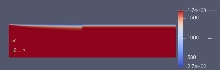
../../../../../_images/initial_temperature.png — Fig. 68 Initial temperature condition for the lazy-expression syntax cookbook.#

The structure and refinement of the mesh are determined in two subsections of the parameter file. First, because the model domain is not a square, it is necessary to subdivide the domain into sections that are equidimensional (or as close as possible): this is done using the repetitions parameters in the Geometry section. In this case because the model domain has an aspect ratio of 5:1, we use 5 repetitions in the \(x\) direction, dividing the domain into 5 equidimensional elements each 1000 by 1000 km.

# Want a 2D box 5000 km wide by 1000 km deep (5e6 x 1e6  meters)
# The variable repetitions divides the whole domain into 5 boxes (1000 x 1000 km)
# as the 0th level mesh refinement: this is needed so elements are squares
# and not elongated rectangles.

subsection Geometry model
  set Model name = box

  subsection Box
    set X extent = 5e6
    set Y extent = 1e6
    set X repetitions = 5
    set Y repetitions = 1
  end
end

Further refinements will divide each sub-region multiple times keeping the aspect ratio of the sub-region. In this case, we refine the elements in each subregion 3 more times. We then use the minimum refinement function strategy and use the if-then-else statement in the function expression to refine 4 more times to a refinement level of 7, but only where the depth is less than 150 km. Appropriate values of the minimum refinement level in this function expression could be the sum of initial global refinement level (3) and initial adaptive refinement level (4) in the ‘then’ statement (i.e., 7 here) and the value of initial global refinement in the ‘else’ statement.

# Refine the upper 150 km of the mesh so lithosphere structure is resolved.
# Function expression asks if the depth is less than the lithosphere depth and
# then refinement level = 7, else refinement level = 0.
# Note, the minimum refinement level for the lower 850 km of the mesh would be
# coarser than the initial one level of global refinement. This would then lead
# to coarsening in the future.
# To avoid this, you may want to set this 'else' value to the same as the number
# of initial global refinement steps.

subsection Mesh refinement
  set Initial global refinement          = 3
  set Minimum refinement level           = 3
  set Initial adaptive refinement        = 4
  set Time steps between mesh refinement = 1
  set Strategy                           = minimum refinement function

  subsection Minimum refinement function
    set Coordinate system   = cartesian
    set Variable names      = x,y
    set Function constants  = ymax=1.e6, lith=1.5e5
    set Function expression = ((ymax-y<=lith) ? 7 : 0)
  end
end

Fig. 69 zooms in on the region where the two plates meet and shows the temperature on a wireframe highlighting the element size refinement. Notice that the mesh refinement algorithm automatically adjusts the element size between the region that is specific to be a level 7 and the region at level 3 to create a smooth transition in element size.

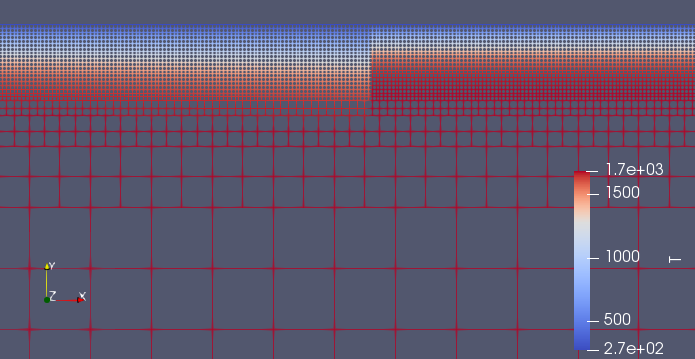
../../../../../_images/initial_temperature_on_mesh_zoom.png — Fig. 69 Initial temperature condition for the lazy-expression syntax cookbook within the region where the two plates meet. The wireframe shows the element size refinement.#

Finally, in order to just test whether the initial temperature structure has been properly defined, it is helpful to run the model for a single time-step and without actually waiting for the solvers to converge. In order to do this, the End time can be set to zero. If the model is very large (lots of refinement) or there are large viscosity jumps that take longer to converge in the Stokes solver, it can also be useful to set the solver tolerance parameters to large values as noted below. However, remember that in that case the solution will not be converged – it is only useful for checking that the initial condition is set correctly.

# Dimension, end-time (years) and output directory
# Only does zeroth time-step to show that initial condition works

set Dimension                              = 2
set Use years in output instead of seconds = true
set Start time                             = 0
set End time                               = 0

# If you have a large model or a model with large viscosity variation and you
# want to run the 0th timestep more quickly in order to just check in the initial
# condition (IC), you can set these solver tolerance values to larger numbers, but
# this means the solution will not be converged.

subsection Solver parameters
  subsection Stokes solver parameters
    set Linear solver tolerance            = 1e-6 # can set to 1e-3 for checking IC
  end
end