Using active particles.#
In the examples above, particle properties passively track distinct model properties. These particle properties, however, may also be used to actively influence the model as it runs. For instance, a composition-dependent material model may use particles’ initial composition rather than an advected compositional field. To make this work – i.e., to get information from particles that are located at unpredictable locations, to the quadrature points at which material models and other parts of the code need to evaluate these properties – we need to somehow get the values from particles back to fields that can then be evaluated at any point where this is necessary. A slightly modified version of the active-composition cookbook (cookbooks/composition_active/composition_active.prm) illustrates how to use ‘active particles’ in this manner.
This cookbook,
cookbooks/composition_active_particles/composition_active_particles.prm,
modifies two sections of the input file. First, particles are added under the
Postprocess section:
subsection Postprocess
  subsection Particles
    set Number of particles         = 100000
    set Time between data output  = 0
    set Data output format        = vtu
    set List of particle properties = velocity, initial composition
    set Interpolation scheme      = cell average
    set Particle generator name   = random uniform
  end
end
Here, each particle will carry the velocity and initial composition
properties. In order to use the particle initial composition value to modify
the flow through the material model, we now modify the Composition section:
subsection Compositional fields
  set Number of fields            = 2
  set Names of fields             = lower, upper
  set Compositional field methods = particles, particles
  set Mapped particle properties  = lower:initial lower, upper:initial upper
end
What this does is the following: It says that there will be two compositional
fields, called lower and upper (because we will use them to indicate
material that comes from either the lower or upper part of the domain). Next,
the Compositional field methods states that each of these fields will be
computed by interpolation from the particles (if we had left this parameter at
its default value, field, for each field, then it would have solved an
advection PDE in each time step, as we have done in all previous examples).
In this case, we specify that both of the compositional fields are in fact
interpolated from particle properties in each time step. How this is done is
described in the fourth line. To understand it, it is important to realize
that particles and fields have matching names: We have named the fields
lower and upper, whereas the properties that result from the
initial composition entry in the particles section are called
initial lower and initial upper, since they inherit the names of the
fields.
The syntax for interpolation from particles to fields then states that the
lower field will be set to the interpolated value of the initial lower
particle property when solving for the composition, and similarly for the upper
field. In turn, the initial composition particle property was using the same
method that one would have used for the compositional field initialization if
these fields were actually advected along in each time step.
In this model the given global refinement level (5), associated number of cells (1024) and 100,000 total particles produces an average particle-per-cell count slightly below 100. While on the high end compared to most geodynamic studies using active particles, increasing the number of particles per cell further may alter the solution. As with the numerical resolution, any study using active particles should systematically vary the number of particles per cell in order to determine this parameter’s influence on the simulation.

