Convection in a 2d box with a phase transition#
This section was contributed by Juliane Dannberg.
This cookbook shows how to use a phase function formulation to introduce phase transitions in a model, using the setup of Christensen and Yuen [1985] (which was the paper that originally introduced phase functions). The paper includes several different setups; here we only reproduce the incompressible cases using the Boussinesq Approximation.
The model setup is a 2d quadratic box with prescribed temperatures at the top and bottom, insulating side walls, and free slip conditions on all boundaries. All material properties are constant, except for the density, which depends on temperature and on the stable phase. There is one phase transition in the center of the model domain (at a depth of 675 km), and the stable phase is represented by the phase function
which defines the fraction of the material that has already undergone the transition to the denser phase and takes the shape of a hyperbolic tangent. The phase function is 0 above the transition, and 1 below the transition. Here, \(p_h\) is the hydrostatic pressure, \(\gamma = -2.7~\text{ MPa K}^{-1}\) is the Clapeyron slope of the phase transition, \(\rho_0 = 1000~\text{ kg m}^{-3}\) is the reference density, \(g = 10~\text{ m s}^{-2}\) is the magnitude of the gravitational acceleration, and \(d = 67.5~\text{ km}\) is the half-thickness of the phase transition (corresponding to 5% of the height of the box).
In the model series presented in Christensen and Yuen [1985], two important parameters are varied: the Rayleigh number (see for example Convection in a 2d box), which takes the values \(Ra = 10^4\), \(10^5\), \(4 \times 10^5\) and \(2 \times 10^6\), and the phase buoyancy parameter, which is controlled by the Clapeyron slope of the phase transition (see Christensen and Yuen [1985]) and takes values between \(-0.8\) and \(0.4\). For a negative Clapeyron slope/phase buoyancy, the phase transition impedes flow; for a positive Clapeyron slope/phase buoyancy, the phase transition accelerates flow.
In order to set up this model in ASPECT, we use the latent heat material model, which includes an implementation of the phase function formulation. The model in Christensen and Yuen [1985] is nondimensional, but we want to use Earth-like parameters here. To achieve this, we set most material properties to multiples of 10, and then control the three important model parameters by setting
the thermal conductivity to \(k = 2.460375 \times 10^7 / Ra~\text{ W m}^{-1}\text{ K}^{-1}\), to set the Rayleigh number,
the Clapeyron slope to \(\gamma = P (Ra/Rb) (\rho_0 g h/\Delta T) = P/2 \times 1.35 \times 10^7~\text{ Pa K}^{-1}\) Pa/K, to set the phase buoyancy parameter \(P\) (where \(Rb\) is the boundary Rayleigh number, defined analogous to the Rayleigh number as \(Rb = \Delta \rho g h^3 / \kappa \eta\), \(h=1350~\text{ km}\) is the height of the box, and \(\Delta T = 1000~\text{ K}\) is the temperature difference between the top and bottom of the box), and
the density change across the phase transition to \(\Delta \rho = 2 \alpha \rho_0 \Delta T = 200~\text{ kg m}^{-3}\), to achieve \(Rb\) = 2\(Ra\) (where \(\alpha = 10^{-4}~\text{ K}^{-1}\) is the thermal expansivity).
Our input file is for a Rayleigh number of \(Ra = 10^5\) and a phase buoyancy parameter of \(P=-0.4\). The material properties are therefore set as follows:
subsection Material model
  set Model name = latent heat
  set Material averaging = harmonic average only viscosity

  subsection Latent heat
    # All parameters in the equation of state are constant, and the mode is incompressible.
    set Reference temperature                          = 500
    set Reference density                              = 1000
    set Reference specific heat                        = 1000
    set Thermal expansion coefficient                  = 1e-4
    set Compressibility                                = 0
    set Thermal conductivity                           = 246.03750       # k = 2.460375e7/Ra, corresponds to Ra = 1e5

    # There is one phase transition in the center of the box (at a depth of 675 km),
    # with a width of 67.5 km (5% of the box height).
    # It occurs at that depth if the temperature corresponds to the reference temperature (500 K);
    # for different temperatures the depth changes according to the Clapeyron slope (-2.7 MPa/K).
    # At the phase transition, the density increases from its reference value of 1000 kg/m^3 to
    # 1200 kg/m^3.
    set Define transition by depth instead of pressure = true
    set Phase transition depths                        = 675000
    set Phase transition widths                        = 67500
    set Phase transition temperatures                  = 500
    set Phase transition Clapeyron slopes              = -2700000        # gamma = P * Ra/Rb, corresponds to P = -0.4
    set Phase transition density jumps                 = 200             # deltarho = 2 alpha rho DeltaT (Rb = 2Ra)
    set Corresponding phase for density jump           = 0

    # The viscosity is constant
    set Viscosity                                      = 1e20
    set Minimum viscosity                              = 1e20
    set Maximum viscosity                              = 1e20
    set Viscosity prefactors                           = 1,1
    set Thermal viscosity exponent                     = 0.0
  end
end
We run the model until a steady state heat flow is reached, or, in case the model does not reach steady state, until a time of 200 Myr. Depending on the Rayleigh number and the phase buoyancy parameter, the flow pattern in steady state can be very different: For positive or low negative Clapeyron slopes, one large convection cell develops. The more negative the Clapeyron slope of the phase transition, the more it impedes the flow, leading to episodic, or completely layered convection (see Fig. 70).
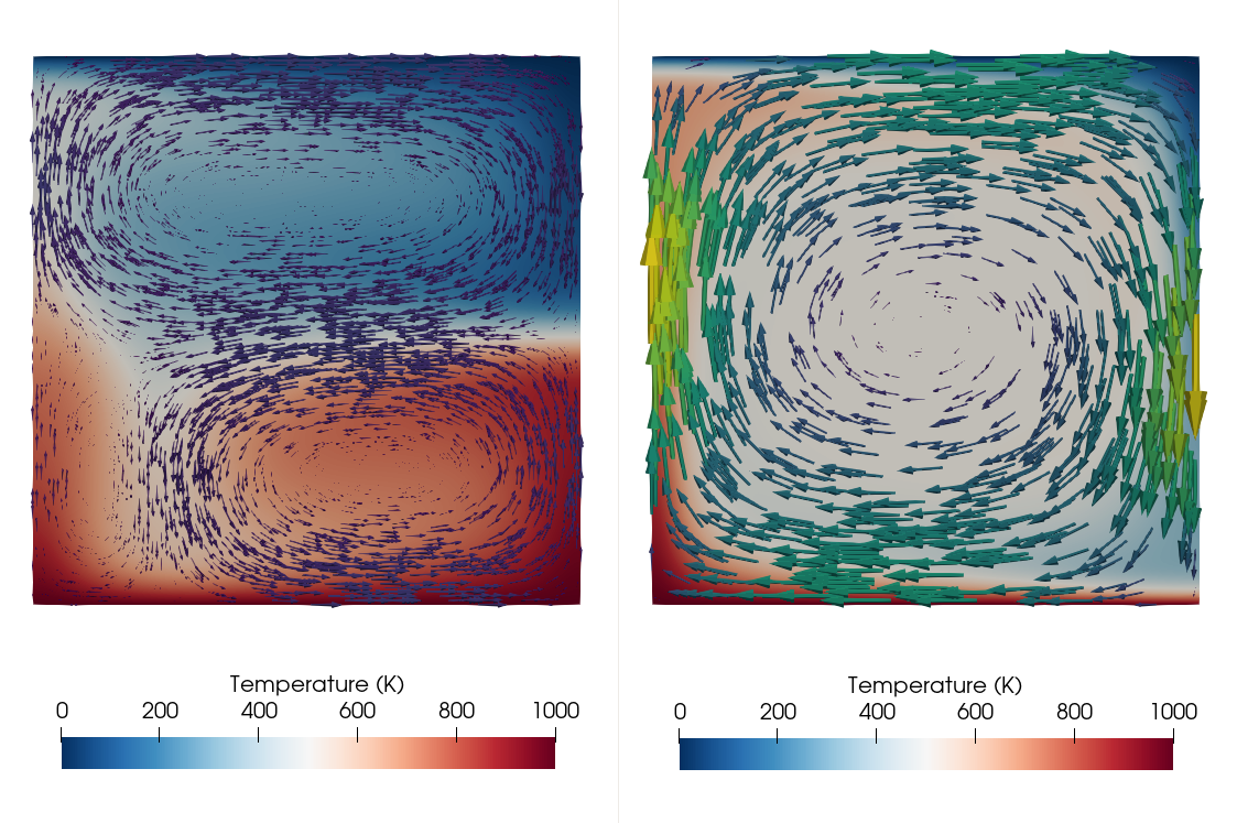
Fig. 70 Phase function model: Flow field in steady state for two models with a Rayleigh number of Ra \(= 10^5\), but different phase buoyancy. The model on the left has a Clapeyron slope of \(-2.7~\text{ MPa K}^{-1}\) (corresponding to \(P=-0.4\)) as in the original input file, leading to layered convection. The model on the right has a Clapeyron slope of \(+2.7~\text{ MPa K}^{-1}\) (corresponding to \(P=0.4\)), leading to one large convection cell.#
The shell script run_all_models.sh in the same folder can be used to run the
whole model series of Boussinesq cases presented in Christensen and Yuen [1985].