Mantle convection using tomography data

This section was contributed by Arushi Saxena, Juliane Dannberg and René Gassmöller

Mantle flow models based on present-day observational constraints can help us to investigate several global and regional tectonic processes. This cookbook describes how to set up such a model based on input tomography data and plate boundary locations. These models are typically computationally very expensive in 3D to make meaningful comparisons with the observations, therefore, we explain the workflow for a 2D spherical shell.

Description of input files

In this cookbook, the input tomography data uses the LLNL-G3D-JPS model [Simmons et al., 2019], available at the IRIS DMC webpage, read in as an ASCII compositional data file. The input file is located in cookbooks/tomography_based_plate_motions/input_data/ and has the following format

# Columns: 
# r     phi    theta  grain_size Vp      Vs     Vs_anomaly faults cratons
3478512 0.0000 0.0000 0.005      13627.1 7185.7 -0.0053    0      0
3598454 0.0000 0.0000 0.005      13598.3 7201.4 -0.0053    0      0
3698402 0.0000 0.0000 0.005      13507.5 7205.6 -0.0053    0      0
3898289 0.0000 0.0000 0.005      13298.2 7077.8 -0.0013    0      0

where grain_size is set to a constant value of 5mm, Vp and Vs are the P- and S-wave seismic velocities, respectively, Vs_anomaly is the S-wave velocity anomaly relative to a reference velocity profile, faults represent the composition value at plate boundaries, and cratons represent the composition value within the continental cratons. Both faults and cratons have composition values set to 0 in this ASCII file because they are defined separately using the Geodynamics World Builder (GWB) [Fraters et al., 2019] and the input file cookbooks/tomography_based_plate_motions/input_file/world_builder_smac_cratons_faults_2D.json.

For defining plate boundary geometry, we use the Nuvel model [DeMets et al., 1990] input as “fault” features and the locations of cratons taken from [Nataf and Ricard, 1996] input as “continental plate” features in GWB [Fraters et al., 2019]. The compositional value of faults transitions smoothly from 1 at the fault trace to 0 over a width of 50 km on either side of the fault. We do this to ensure that the prescribed plate boundary viscosity which is based on the fault composition is also smooth. Note that while the input file includes plate boundary geometry and cratons for the whole Earth, we only compute the compositions along a cross-section in this cookbook. The input faults and cratons in a 3D spherical model would look like Fig. 138.

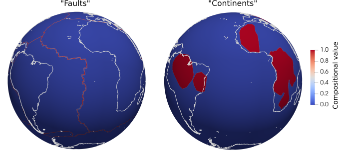
Fig. 138 The composition of plate boundary geometry (“faults”) and cratons (“continents”) using the input file coordinates for a 3D model.

Computed material properties

A common practice in mantle convection models using tomography data is to use a different model for the uppermost mantle structure because of the limited seimic resolution to accurately resolve the lithospheric structure and slabs. For this cookbook, we use a temperature model, TM1 [Osei Tutu et al., 2018], located in cookbooks/tomography_based_plate_motions/input_data/upper_mantle_TM1_2D.txt. The user can control the depth until which we want to use this temperature model using the uppermost mantle thickness parameter. Fig. 139 shows the input Vs anomalies and the computed temperatures in the model.

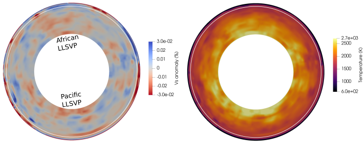
Fig. 139 The input Vs anomalies (left) and the computed temperatures (right). Note that we only use tomography-based temperatures below the uppermost mantle thickness depth, marked by the white contour line.

We compute the density from the thermal anomalies in the TM1 model relative to a reference temperature of 293 K as done by Osei Tutu et al. [2018]. We use constant thermal expansion coefficients and compressibilities within the crust, lithospheric mantle and asthenosphere, respectively. To define the crust and the lithosphere, we use the lithospheric thickness from Priestley et al. [2018] and crustal thicknesses from the crust1.0 model [Laske et al., 2012].

Below “uppermost mantle thickness”, the temperature and the density fields are computed using the corresponding depth-dependent scaling values taken from [Steinberger and Calderwood, 2006] relative to the input Vs anomalies (compositional field Vs_anomaly), using the scaling files dT_vs_scaling.txt and rho_vs_scaling.txt, respectively, located in cookbooks/tomography_based_plate_motions/input_data/.

In order to avoid jumps in the temperature distribution, we smooth the temperatures between the two models across the “uppermost mantle thickness” depth using a sigmoid function with a half-width of 20km.

The viscosity in the model follows a dislocation diffusion creep law with prefactors, activation energies and volumes for major phase transitions. Additionally, we scale the laterally averaged viscosity to a reference viscosity profile from the profile of Steinberger and Calderwood [2006]. The user can choose from the available reference viscosity profiles in the cookbooks/tomography_based_plate_motions/input_data/viscosity_profiles folder. The model defines different viscosities at the plate boundaries and within the cratonic regions. For Earth-like behavior, plate boundaries and cratons have reduced and increased viscosity, respectively, compared to the surrounding lithosphere.

Running the model

The plugin that implements the material properties described above is tomography_based_plate_motions.cc located in the cookbooks/tomography_based_plate_motions/plugins directory, and can be compiled with cmake . && make in this directory. The model can then be run using the prm file 2D_slice_with_faults_and_cratons.prm. The sections relevant to this cookbook are:

subsection Compositional fields
  set Number of fields = 6
  set Names of fields = grain_size, Vp, Vs, vs_anomaly, faults, continents
  set Compositional field methods = static, static, static, static, static, static
end

subsection Initial composition model
  set List of model names = ascii data, world builder

  subsection Ascii data model
    set Data directory = ../../input_data/
    set Data file name = LLNL_model_cropped_cratons_faults.txt.gz
    set Slice dataset in 2D plane = true
  end

  subsection World builder
    set List of relevant compositions = faults, continents
  end
end

subsection Temperature field
  set Temperature method = prescribed field
end

subsection Material model
  set Model name         = tomography based plate motions
  set Material averaging = harmonic average only viscosity

  subsection Tomography based plate motions model
   set Uppermost mantle thickness                  = 300000

   set Use depth dependent viscosity               = true
   subsection Ascii data model
     set Data directory                            = ../../input_data/viscosity_profiles/
     set Data file name                            = steinberger_source-1.txt
   end

   set Use depth dependent density scaling         = true
   set Use depth dependent temperature scaling     = true
   subsection Density velocity scaling
     set Data file name                            = rho_vs_scaling.txt
   end
   subsection Temperature velocity scaling
     set Data file name                            = dT_vs_scaling.txt
   end

   set Use faults                                  = true
   set Fault viscosity                             = 1e19
   set Use cratons                                 = true
   set Craton viscosity                            = 1e25

   set Asthenosphere viscosity                     = 1e20
  end
end

After running this model, we can visualize the computed material properties and analyze the instantaneous mantle flow. Fig. 140 shows the computed non-adiabatic density and viscosity fields in the model along with the velocities generated from the force balance between driving and resisting forces.

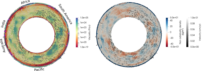
Fig. 140 Instantaneous velocity field in the model overlying the heterogeneous lateral and radial viscosity distribution (left) and the non-adiabatic densities (right). The magenta and white contours represent the compositional field corresponding to plate boundaries and cratons, respectively. The cyan contour marks the lithospheric depths in our model, which also controls the depth until which the viscosities at the plate boundaries extend.

It is difficult to compare the modeled surface deformation with the observations using a 2D shell, but we can already see the expected flow patterns such as upwellings due the positive buoyancy beneath the African plate and downwellings due to slabs under the Pacific plate.

The user can change several parameters to investigate the mantle forces and how they affect the flow, such as:

• The input tomography model, several options are available on the IRIS DMC webpage.

• The density or temperature scaling relative to the input shear wave anomalies.

• The reference viscosity profile.

• The prescribed viscosity of the plate boundaries, which controls friction between plates.

• To use viscous and neutrally buoyant cratons in the model.