Lower crust flow with an obstacle#
This section was contributed by Cedric Thieulot.
The setup for this experiment originates in Clark et al. [2005] in which the authors model dynamic stresses associated with the obstruction of lower crustal channel flow due to rheological heterogeneity in Eastern Tibet. They compare model calculations with observed topography where they interpret channel flow of the deep crust to be inhibited by the rigid Sichuan Basin as illustrated in Fig. 107 and Fig. 108.
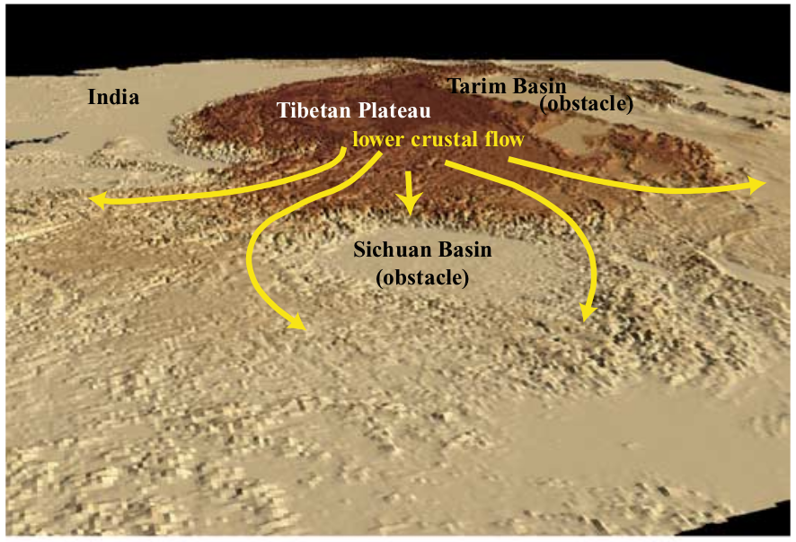
Fig. 107 3-D perspective of digital topography of eastern and southeastern Tibet, view to the west and northwest. Taken from Clark et al. [2005].#
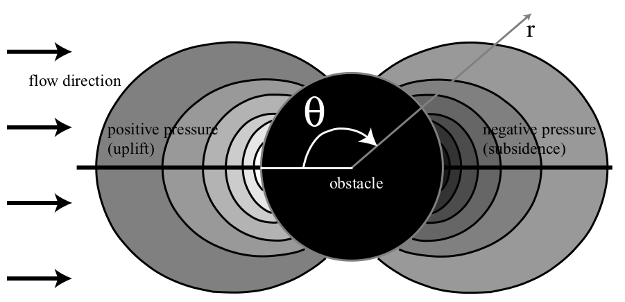
Fig. 108 General model showing map-view patterns of high and low dynamic pressures. Background flow is from left to right. Positive dynamic pressure (i.e. a load acting upwards on the top of the channel) is observed ‘upstream’ of the flow direction and predicts uplift at the surface. Taken from Clark et al. [2005].#
A discussion of this model in the context of Eastern Tibet is provided in Pitard et al. [2023].
The domain is a 3D Cartesian box of size \((L_x,L_y,L_z) = (1000~\text{km}, 500~\text{km}, 15~\text{km})\). Gravity is set to zero so that density values are of no importance. Boundary conditions are no-slip at the top (\(z=0\)) and bottom (\(z=L_z\)), free slip on the \(y=0\) and \(y=L_y\) sides, and a parabolic Poiseuille flow velocity \(v_x(z)\) is prescribed on the \(x=0\) and \(x=L_x\) sides:
with \(U_0=80~\text{ mm year}^{-1}\). The authors justify this by stating: Flow within the channel is driven by horizontal pressure gradients, due to topographic gradients and variations in crustal thickness or density. In reality, flowing lower crustal material is likely not to have sharp, well-defined channel boundaries, but most geodynamic models approximate flow behaviour as Poiseuille flow.
Temperature plays no role here and fluids are assumed to be Newtonian. Because of the symmetry of the problem, we only model half of it, and the obstacle is a half vertical cylinder centered at location \((x,y) = (L_x/2,0)\) and has a radius of \(200~\text{km}\). The obstacle has a viscosity of \(2\cdot 10^{21}~\text{ Pa s}\) which is 1000 times larger than the viscosity of the lower crust \(2\cdot 10^{18}~\text{ Pa s}\).
Because kinematical boundary conditions are prescribed on all 6 sides there is a pressure nullspace that is removed by requiring that the average of the pressure over the whole volume is zero.
The viscosity field is shown in Fig. 109
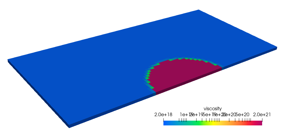
Fig. 109 Viscosity field (Pa.s).#
The velocity field is shown in Fig. 110. It is maximum at \(z=L_z/2\) and zero at the bottom and at the top of the domain, the assumption being that the lower crust flows faster than the upper crust is moving.
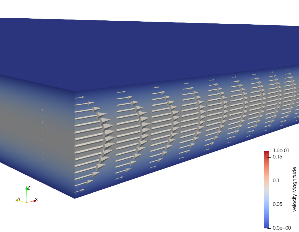
Fig. 110 Velocity field at the \((x=0,y=0)\) corner.#
One can look at the velocity, pressure and strain rate fields on the \(z=L_z/2\) plane, as shown in Fig. 111, Fig. 112 and Fig. 113.
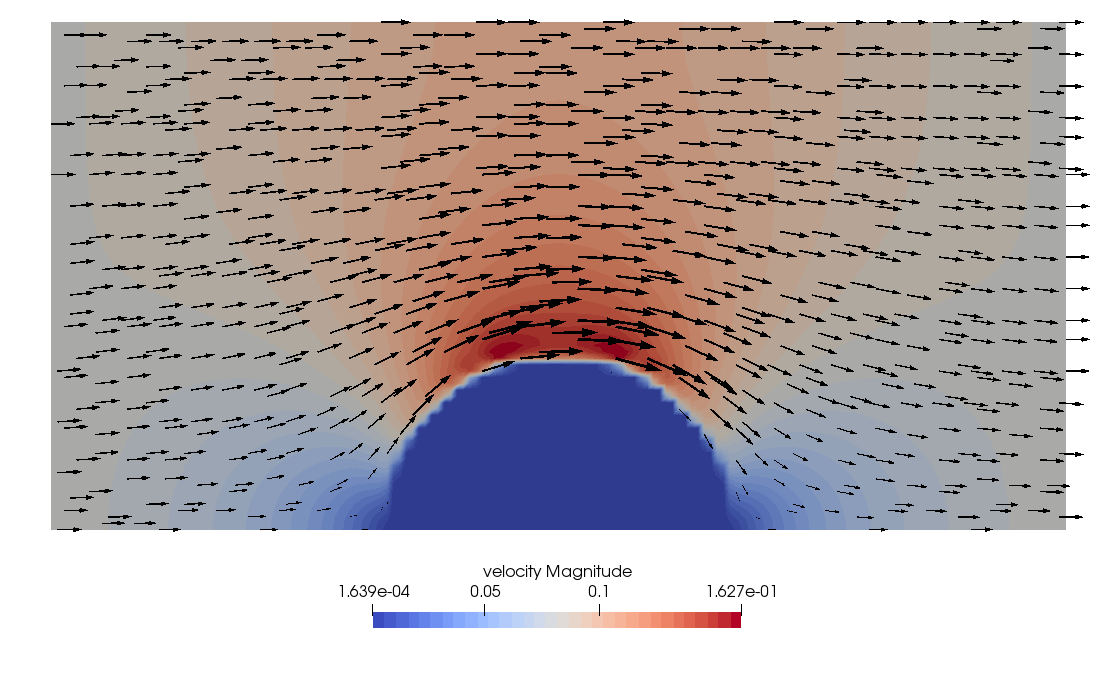
Fig. 111 Velocity field on \(z=L_z/2\) plane.#
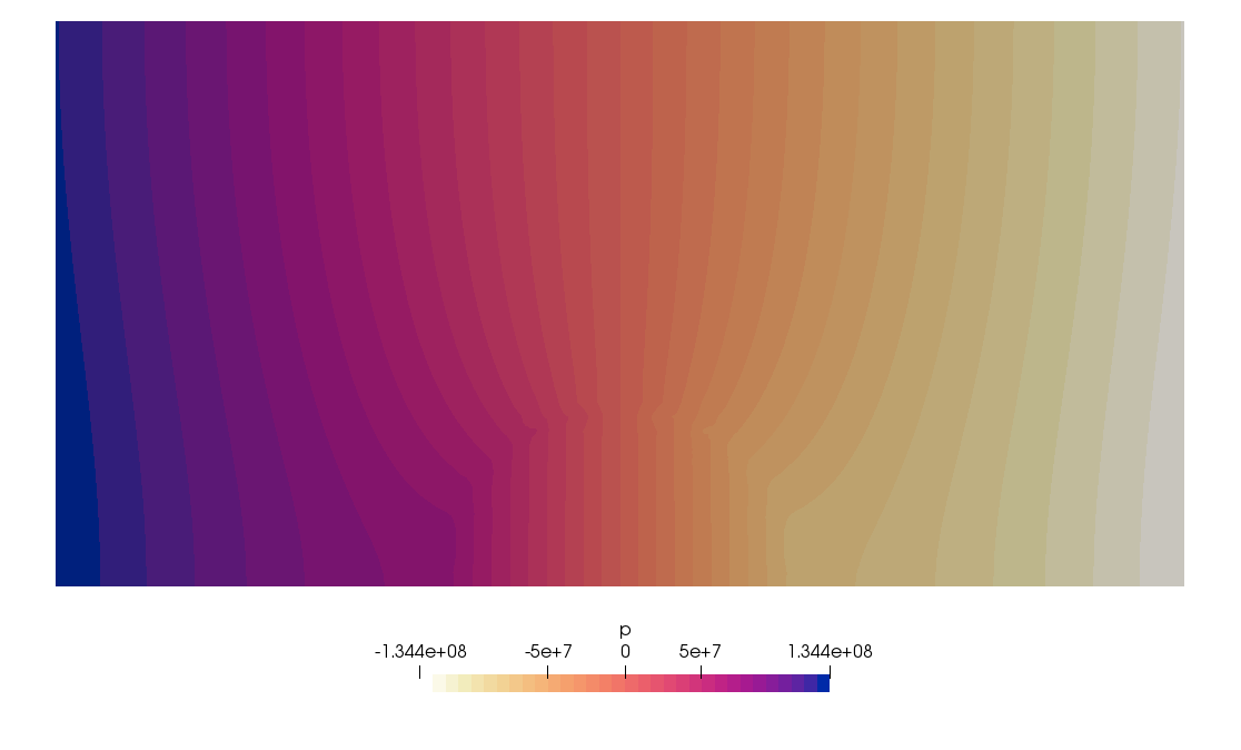
Fig. 112 Pressure field on \(z=L_z/2\) plane.#
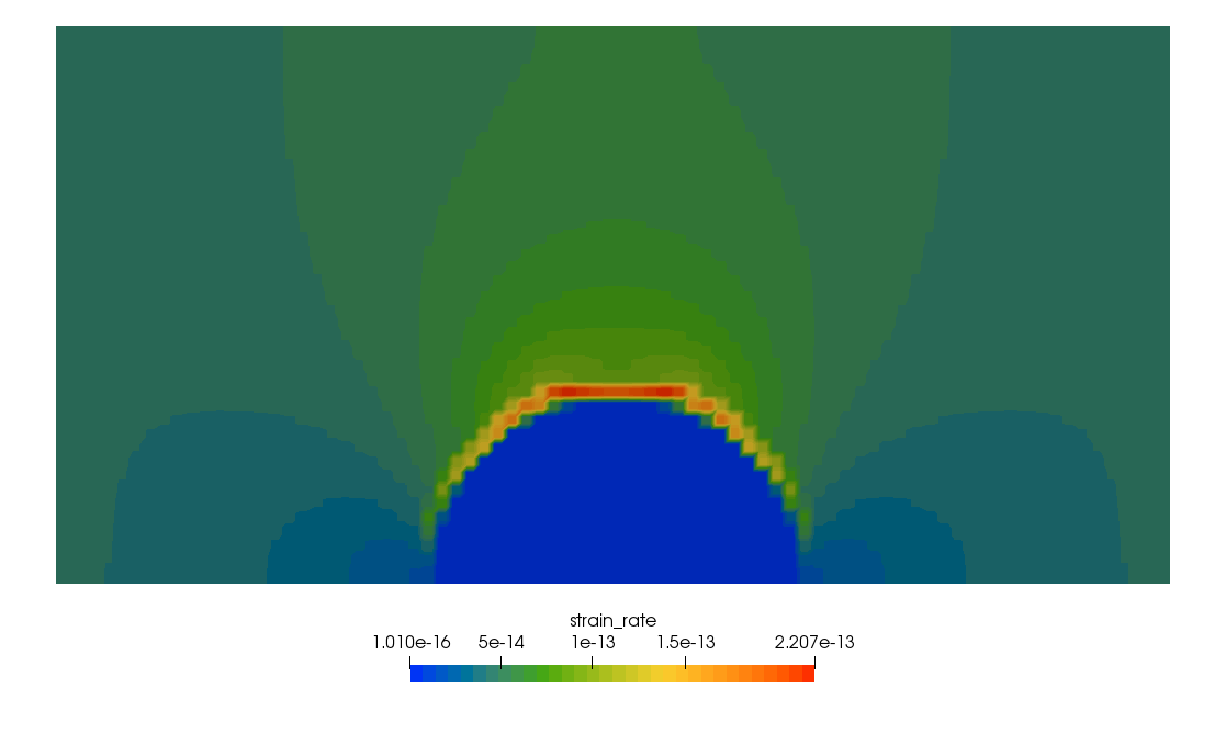
Fig. 113 Strain rate field on \(z=L_z/2\) plane.#
Note that when the viscosity of the obstacle is set to the same viscosity as the flowing crust then the velocity assumes the prescribed parabolic profile everywhere and the pressure is linear and only depends on \(x\).