The 2D cylindrical shell benchmarks by Davies et al.

This section was contributed by William Durkin and Wolfgang Bangerth.

All of the benchmarks presented so far take place in a Cartesian domain. Davies et al. describe a benchmark (in a paper that is currently still being written) for a 2D spherical Earth that is nondimensionalized such that

\(r_{\min}\) = 1.22	\( T |_{r_{min}} = 1\)
\(r_{\max}\) = 2.22	\( T |_{r_{max}} = 0\)

The benchmark is run for a series of approximations (Boussinesq, Extended Boussinesq, Truncated Anelastic Liquid, and Anelastic Liquid), and temperature, velocity, and heat flux calculations are compared with the results of other mantle modeling programs. will output all of these values directly except for the Nusselt number, which we must calculate ourselves from the heat fluxes that can compute. The Nusselt number of the top and bottom surfaces, \({Nu}_T\) and \({Nu}_B\), respectively, are defined by the authors of the benchmarks as

(44)\[{Nu}_{T} = \frac{\ln(f)}{2{\pi}r_{\max}(1-f)}\int \limits_{0}^{2\pi} \frac{\partial T}{\partial r}\, \text{d}\theta\]

and

(45)\[{Nu}_{B} = \frac{f \ln(f)}{2{\pi}r_{\min}(1-f)}\int \limits_{0}^{2\pi} \frac{\partial T}{\partial r}\, \text{d}\theta\]

where \(f\) is the ratio \(\frac{r_{\min}}{r_{\max}}\).

We can put this in terms of heat flux

\[q_r = -k\frac{\partial T}{\partial r}\]

through the inner and outer surfaces, where \(q_r\) is heat flux in the radial direction. Let \(Q\) be the total heat that flows through a surface,

\[Q = \int \limits_{0}^{2\pi} q_r\, \text{d}\theta,\]

then (44) becomes

\[{Nu}_{T} = \frac{-Q_{T}\ln(f)}{2\pi{r_{\max}}(1-f)k}\]

and similarly

\[{Nu}_{B} = \frac{-Q_{B}f\ln(f)}{2\pi{r_{\min}}(1-f)k}.\]

\(Q_T\) and \(Q_B\) are heat fluxes that can readily compute through the heat flux statistics postprocessor (see Parameter name: List of postprocessors). For further details on the nondimensionalization and equations used for each approximation, refer to Davies et al.

The series of benchmarks is then defined by a number of cases relating to the exact equations chosen to model the fluid. We will discuss these in the following.

Case 1.1: BA_Ra104_Iso_ZS.

This case is run with the following settings:

• Boussinesq Approximation

• Boundary Condition: Zero-Slip

• Rayleigh Number = \(10^4\)

• Initial Conditions: \(D = 0, O = 4\)

• \(\eta(T) = 1\)

where \(D\) and \(O\) refer to the degree and order of a spherical harmonic that describes the initial temperature. While the initial conditions matter, what is important here though is that the system evolve to four convective cells since we are only interested in the long term, steady state behavior.

The model is relatively straightforward to set up, basing the input file on that discussed in Section Simple convection in a quarter of a 2d annulus. The full input file can be found at benchmarks/davies_et_al/case-1.1.prm, with the interesting parts excerpted as follows:

############### Parameters describing the model

subsection Geometry model
  set Model name = spherical shell

  subsection Spherical shell
    set Inner radius  = 1.22
    set Opening angle = 360
    set Outer radius  = 2.22
  end
end

# [...]

subsection Material model
  set Model name = simple

  subsection Simple model
    set Reference density             = 1
    set Reference specific heat       = 1.
    set Reference temperature         = 0
    set Thermal conductivity          = 1
    set Thermal expansion coefficient = 1e-6
    set Viscosity                     = 1
  end
end

############### Parameters describing the temperature field
# Angular mode is set to 4 in order to match the number of
# convective cells reported by Davies et al.

subsection Initial temperature model
  set Model name = spherical hexagonal perturbation

  subsection Spherical hexagonal perturbation
    set Angular mode          = 4
    set Rotation offset       = 0
  end
end

############### Prescribe the Rayleigh number as g*alpha
# Here, Ra = 10^4 and alpha was chosen as 10^-6 above.
subsection Gravity model
  set Model name = radial constant

  subsection Radial constant
    set Magnitude =  1e10
  end
end

# [...]

We use the same trick here as in Convection in a 2d box to produce a model in which the density \(\rho(T)\) in the temperature equation (3) is almost constant (namely, by choosing a very small thermal expansion coefficient) as required by the benchmark, and instead prescribe the desired Rayleigh number by choosing a correspondingly large gravity.

Results for this and the other cases are shown below.

Case 2.1: BA_Ra104_Iso_FS.

Case 2.1 uses the following setup, differing only in the boundary conditions:

• Boussinesq Approximation

• Boundary Condition: Free-Slip

• Rayleigh Number = \(10^4\)

• Initial Conditions: \(D = 0, O = 4\)

• \(\eta(T) = 1\)

As a consequence of the free slip boundary conditions, any solid body rotation of the entire system satisfies the Stokes equations with their boundary conditions. In other words, the solution of the problem is not unique: given a solution, adding a solid body rotation yields another solution. We select arbitrarily the one that has no net rotation (see Nullspace removal). The section in the input file that is relevant is then as follows (the full input file resides at benchmarks/davies_et_al/case-2.1.prm):

subsection Nullspace removal
  set Remove nullspace                        = net rotation
end

subsection Boundary temperature model
  set Fixed temperature boundary indicators   = 0,1
end

subsection Boundary velocity model
  set Tangential velocity boundary indicators = 0,1
end

Again, results are shown below.

Case 2.2: BA_Ra105_Iso_FS.

Case 2.2 is described as follows:

• Boussinesq Approximation

• Boundary Condition: Free-Slip

• Rayleigh Number = \(10^5\)

• Initial Conditions: Final conditions of case 2.1 (BA_Ra104_Iso_FS)

• \(\eta(T) = 1\)

In other words, we have an increased Rayleigh number and begin with the final steady state of case 2.1. To start the model where case 2.1 left off, the input file of case 2.1, benchmarks/davies_et_al/case-2.1.prm, instructs to checkpoint itself every few time steps (see Checkpoint/restart support). If case 2.2 uses the same output directory, we can then resume the computations from this checkpoint with an input file that prescribes a different Rayleigh number and a later input time:

############### Global parameters
# Case 2.2 begins with the final steady state solution of Case 2.1
# "Resume computation" must be set to true, and "Output directory" must
# point to the folder that contains the results of Case 2.1.

set CFL number                             = 10
set End time                               = 3
set Output directory                       = output
set Resume computation                     = true

We increase the Rayleigh number to \(10^5\) by increasing the magnitude of gravity in the input file. The full script for case 2.2 is located in benchmarks/davies_et_al/case-2.2.prm

Case 2.3: BA_Ra103_vv_FS.

Case 2.3 is a variation on the previous one:

• Boussinesq Approximation

• Boundary Condition: Free-Slip

• Rayleigh Number = \(10^3\)

• Initial Conditions: Final conditions of case 2.1 (BA_Ra104_Iso_FS)

• \(\eta(T) = 1000^{-T}\)

The Rayleigh number is smaller here (and is selected using the gravity parameter in the input file, as before), but the more important change is that the viscosity is now a function of temperature. At the time of writing, there is no material model that would implement such a viscosity, so we create a plugin that does so for us (see Extending and contributing to ASPECT and How to write a plugin in general, and Material models for material models in particular). The code for it is located in benchmarks/davies_et_al/case-2.3-plugin/VoT.cc (where “VoT” is short for “viscosity as a function of temperature”) and is essentially a copy of the simpler material model. The primary change compared to the simpler material model is the line about the viscosity in the following function:

template <int dim>
void
VoT<dim>::
evaluate(const typename Interface<dim>::MaterialModelInputs &in,
         typename Interface<dim>::MaterialModelOutputs &out) const
{
  for (unsigned int i=0; i<in.position.size(); ++i)
    {
      out.viscosities[i] = eta*std::pow(1000,(-in.temperature[i]));
      out.densities[i] = reference_rho * (1.0 - thermal_alpha * (in.temperature[i] - reference_T));
      out.thermal_expansion_coefficients[i] = thermal_alpha;
      out.specific_heat[i] = reference_specific_heat;
      out.thermal_conductivities[i] = k_value;
      out.compressibilities[i] = 0.0;
    }
}

Using the method described in Sections Running benchmarks that require code and How to write a plugin, and the files in the benchmarks/davies_et_al/case-2.3-plugin, we can compile our new material model into a shared library that we can then reference from the input file. The complete input file for case 2.3 is located in benchmarks/davies_et_al/case-2.3.prm and contains among others the following parts:

set Additional shared libraries            = ./case-2.3-plugin/libVoT.so

subsection Material model
  set Model name = VoT

  subsection VoT model
    set Reference density             = 1
    set Reference specific heat       = 1.
    set Reference temperature         = 0
    set Thermal conductivity          = 1
    set Thermal expansion coefficient = 1e-5
    set Viscosity                     = 1
  end
end

Results.

In the following, let us discuss some of the results of the benchmark setups discussed above. First, the final steady state temperature fields are shown in Fig. 201. It is immediately obvious how the different Rayleigh numbers affect the width of the plumes. If one imagines a setup with constant gravity, constant inner and outer temperatures and constant thermal expansion coefficient (this is not how we describe it in the input files, but we could have done so and it is closer to how we intuit about fluids than adjusting the gravity), then the Rayleigh number is inversely proportional to the viscosity – and it is immediately clear that larger Rayleigh numbers (corresponding to lower viscosities) then lead to thinner plumes. This is nicely reflected in the visualizations.

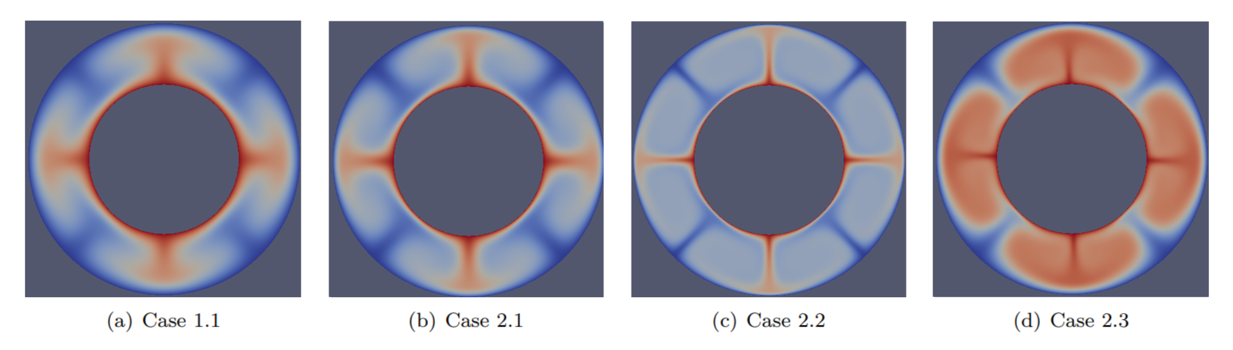
Fig. 201 Davies et al. benchmarks: Final steady state temperature fields for the 2D cylindrical benchmark cases.

Secondly, Fig. 202 shows the root mean square velocity as a function of time for the various cases. It is obvious that they all converge to steady state solutions. However, there is an initial transient stage and, in cases 2.2 and 2.3, a sudden jolt to the system at the time where we switch from the model used to compute up to time \(t=2\) to the different models used after that.

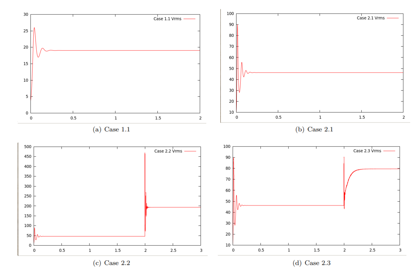
Fig. 202 Davies et al. benchmarks: \(V_{rms}\) for 2D Cylindrical Cases. Large jumps occur when transitioning from case 2.1 to cases 2.2 and 2.3 due to the instantaneous change of parameter settings.

These runs also produce quantitative data that will be published along with the concise descriptions of the benchmarks and a comparison with other codes. In particular, some of the criteria listed above to judge the accuracy of results are listed in Table 10.[1]

Table 10 Davies et al. benchmarks: Numerical results for some of the output quantities required by the benchmarks and the various cases considered.

Case	\(\left<T\right>\)	\(Nu_T\)	\(Nu_B\)	\(V_{\text{rms}}\)
1.1	0.403	2.464	2.468	19.053
2.1	0.382	4.7000	4.706	46.244
2.2	0.382	9.548	9.584	193.371
2.3	0.582	5.102	5.121	79.632

---

[1]

The input files available in the benchmarks/davies_et_al directory use 5 global refinements in order to provide cases that can be run without excessive trouble on a normal computer. However, this is not enough to achieve reasonable accuracy and both the data shown below and the data submitted to the benchmarking effort uses 7 global refinement steps, corresponding to a mesh with 1536 cells in tangential and 128 cells in radial direction. Computing on such meshes is not cheap, as it leads to a problem size of more than 2.5 million unknowns. It is best done using a parallel computation.