
Kinematically-driven 2d oceanic subduction#
This section was contributed by Anne Glerum and Yingying Li.
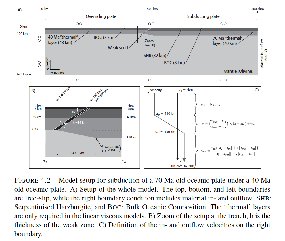
This subduction example is based on the benchmark effort of Quinquis et al., of which initial results were published in Quinquis [2014]. In four increasingly complex cases we will go from isoviscous materials without any temperature effects to a fully thermo-mechanical, nonlinear, strain-weakened visco-plastic, externally-driven model of oceanic subduction. The setup is outlined in Fig. 132. The models are run for 15 My and slab tip depth, trench location, root-mean-square (RMS) velocity and temperature, and viscous dissipation are monitored. In addition, we will discuss the effects of the element size of the subduction interface and crustal layers, viscosity averaging and the solver tolerance.
Case 1: Simple rheology#
The Case 1 model setup considers seven materials (compositional fields) apart from the background sublithospheric mantle (see Fig. 133), including (1) the Bulk Oceanic Composition (BOC), (2) Serpentinized HarzBurgite (SHB) and (3) “thermal” layer of the overriding plate (OP), (4) the BOC, (5) SHB and (6) “thermal” layer of the subducting plate (SP), and (7) the weak seed.
The geometry of these compositions is implemented as follows:
# We fix composition on the right boundary,
# because we have inflow there.
subsection Boundary composition model
set Fixed composition boundary indicators = right
set List of model names = initial composition
end
# The overriding plate (OP) and subducting plate (SP)
# are each divided into three different layers:
# a layer of Bulk Oceanic Composition (BOC),
# a layer of Serpentinized HarzBurgite (SHB),
# and a "thermal layer".
subsection Compositional fields
set Number of fields = 7
set Names of fields = BOC_OP, BOC_SP, SHB_OP, SHB_SP, thermal_OP, thermal_SP, WZ
end
subsection Initial composition model
set List of model names = function
subsection Function
set Function constants = Ax=1475600.0, Az=670000.0, \
Bx=1500000.0, Bz=670000.0, \
Cx=1358500.0, Cz=588000.0, \
Dx=1382900.0, Dz=588000.0, \
Ex=1530000.0, Ez=560000.0, \
Fz=663000.0, Gz=662000.0, \
Hz=631000.0, Iz=630000.0
set Function expression = if(z>=Fz&z>=((Az-Cz)/(Ax-Cx)*(x-Cx)+Cz),1,0); \
if(z>=Gz&z<=((Bz-Dz)/(Bx-Dx)*(x-Dx)+Dz),1,0); \
if(z>=Hz&z>=((Az-Cz)/(Ax-Cx)*(x-Cx)+Cz)&z<Fz,1,0); \
if(z>=Iz&z<=((Bz-Dz)/(Bx-Dx)*(x-Dx)+Dz)&z<Gz,1,0); \
if(z>=Cz&z>=((Az-Cz)/(Ax-Cx)*(x-Cx)+Cz)&z<Hz,1,0); \
if((x>=Ex&z>=Ez&z<Iz)|(x<Ex&z<=((Bz-Dz)/(Bx-Dx)*(x-Dx)+Dz)&z<Iz&z>=((Ez-Dz)/(Ex-Dx)*(x-Dx)+Dz)),1,0); \
if(z>=Cz&z>((Bz-Dz)/(Bx-Dx)*(x-Dx)+Dz)&z<((Az-Cz)/(Ax-Cx)*(x-Cx)+Cz),1.5,0)
set Variable names = x,z
end
end
No differences in material properties exist, except for density and viscosity, so we use the multicomponent material model. To keep the boundaries between fields as sharp as possible in terms of viscosity, we use the maximum composition to determine the viscosity in each evaluation point (note that this can be harder on the solver):
set Nonlinear solver scheme = single Advection, single Stokes
subsection Material model
set Model name = multicomponent
subsection Multicomponent
set Reference temperature = 0.0
set Viscosity averaging scheme = maximum composition
# BOC_OP, BOC_SP, SHB_OP, SHB_SP, thermal_OP, thermal_SP, WZ
set Viscosities = 1.e20, 1.e23, 1.e20, 1.e23, 1.e23, 1.e23, 1.e23, 1.e20
set Densities = 3200.0,3250.0,3250.0,3250.0,3250.0,3250.0,3250.0,3250.0
set Thermal conductivities = 1
end
end
Temperature effects are ignored. Subduction is driven by prescribed in- and outflow through the right boundary (with a gradual transition of the flow direction), all other boundaries are free slip. The volume of material that flows in is balanced by the volume that is prescribed to flow out (this is important as the model is incompressible). A weak crust along the plate interface and the subducting lithosphere facilitates subduction. Through the function plugin, we prescribe the in- and outflow:
subsection Boundary velocity model
set Tangential velocity boundary indicators = left, bottom, top
set Prescribed velocity boundary indicators = right x:function
subsection Function
set Function constants = cm=100.0
set Function expression = if(z<540000.0, (600.0/550.0)/cm, \
if(z>560000.0, -5.0/cm, \
((((-600.0/550.0)-5.0)/-20.0)*((z/1000.0)-560.0)+5.0)*(-1.0/cm))); \
0
set Variable names = x,z
end
end
To follow the slab on its descent into the mantle, we use adaptive mesh refinement based on viscosity in combination with the minimum refinement strategy to ensure sufficient resolution in the crust and weak zone that allow the slab to detach from the surface:
# The maximum refinement level will be 6+4 levels,
# corresponding to a maximum resolution of ~700 m.
subsection Mesh refinement
set Initial adaptive refinement = 4
set Initial global refinement = 6
set Minimum refinement level = 6
set Normalize individual refinement criteria = true
set Refinement criteria merge operation = plus
set Coarsening fraction = 0.01
set Refinement fraction = 0.95
set Run postprocessors on initial refinement = false
set Skip solvers on initial refinement = true
set Skip setup initial conditions on initial refinement = true
set Strategy = minimum refinement function, viscosity
set Time steps between mesh refinement = 16
subsection Minimum refinement function
set Coordinate system = depth
set Variable names = x,z,t
set Function constants = vel=150e3, L=100e3, crust=10e3
set Function expression = if(x<crust,10,if(x<L,9,if(x<vel,8,6)))
end
end
To monitor the model evolution, several diagnostic quantities are tracked over time: the depth of the tip of the slab, the position of the trench, the RMS velocity of the slab and the whole model domain, and the viscous dissipation in the slab and total model domain. The computation of trench position is through a plugin called ‘trench_location’. It needs to be compiled as a shared library that can be called from the input file.
subsection Postprocess
set List of postprocessors = visualization, velocity statistics, heating statistics, maximum depth of field, composition velocity statistics, viscous dissipation statistics, trench location
subsection Visualization
set List of output variables = material properties, strain rate, error indicator
set Time between graphical output = 5e5
subsection Material properties
set List of material properties = density, viscosity
end
end
subsection Trench location
set Name of trench compositional field = BOC_OP
end
subsection Composition velocity statistics
set Names of selected compositional fields = BOC_SP, SHB_SP, thermal_SP
end
end
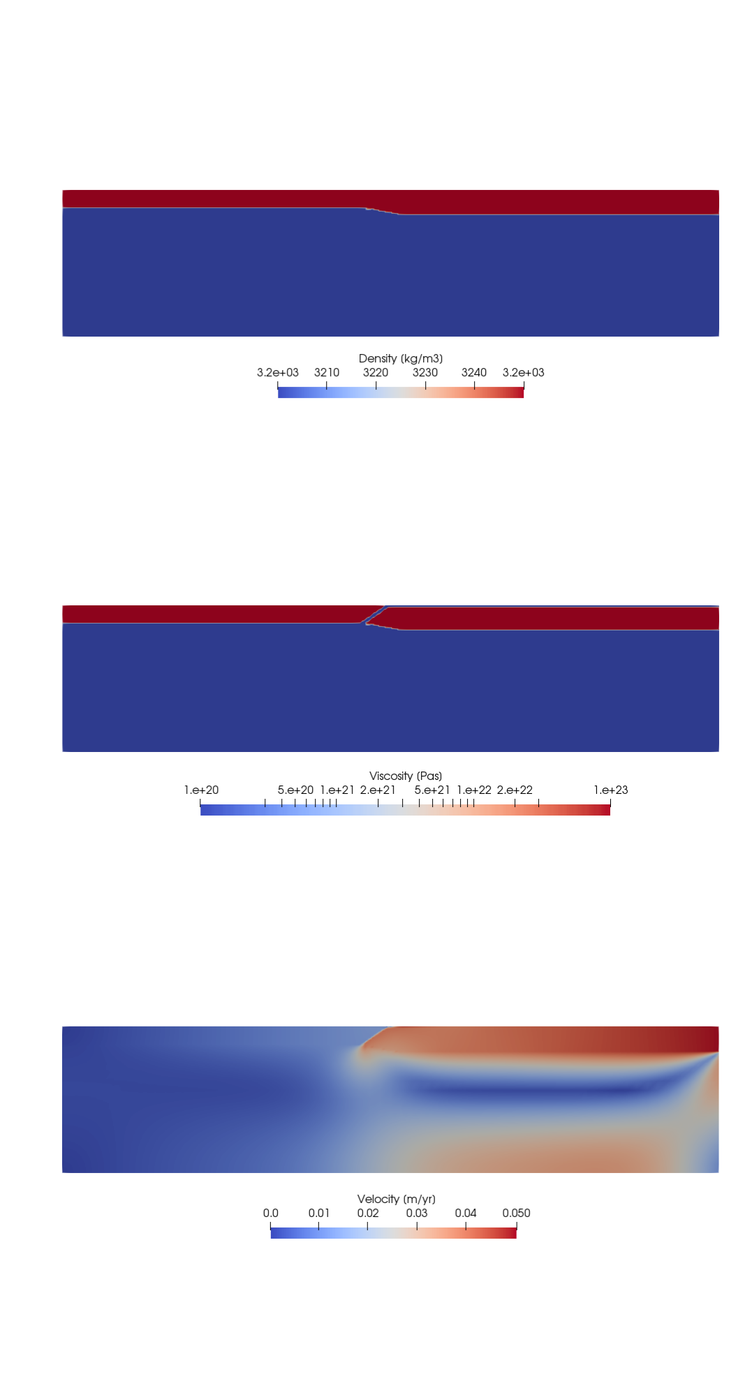
Fig. 133 Case 1 density, viscosity and velocity at time zero.#
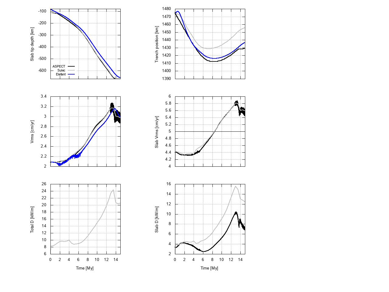
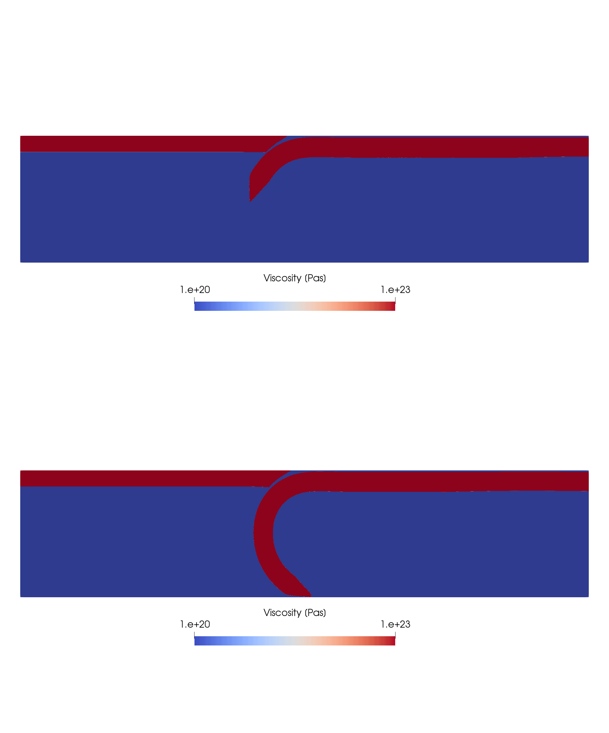
We run the Case 1 setup for 15 My of model time. The diagnostic quantities in Fig. 134 show three stages of model evolution: first trench advance (top right plot), then free subduction (increasing slab RMS velocity), and after about 13 My interaction between the slab and bottom boundary at 660 km depth, which slows down the slab. The slab then curves inward along the bottom boundary. This can also be seen in Fig. 135.
Fig. 134 Case 1 diagnostic quantities of ASPECT#
Fig. 135 Case 1 viscosity snapshots at 8 and 15 My.#
Case 2a: Model with thermal evolution#
Case 2a builds on Case 1 by including a heterogeneous initial temperature field that combines the plate cooling model for the temperature in the plates with an adiabatic temperature gradient below the plates. For the plate cooling model, we assume that the overriding plate is 40 My old and the subducting plate 70 My. The temperature function (including a summation term) is too complex to write out as a function expression in the input file, so it is put in a new initial temperature plugin called ’subduction plate cooling’. This plugin needs to be compiled as a shared library that can be called from the input file:
# We include a shared library with a customized initial temperature plugin and the required isotherm depth, composition RMS temperature, and trench location postprocessors.
set Additional shared libraries = $ASPECT_SOURCE_DIR/cookbooks/kinematically_driven_subduction_2d/libsubduction_plate_cooling.so
# We fix temperature on the top and bottom,
# as well as on the right boundary because
# we have inflow through the latter.
subsection Boundary temperature model
set Fixed temperature boundary indicators = bottom, top, right
set List of model names = box
subsection Box
set Bottom temperature = 0
set Left temperature = 0
set Right temperature = 0
set Top temperature = 0
end
end
subsection Initial temperature model
set List of model names = subduction plate cooling
end
The initial temperature distribution can be seen in Fig. 136
Fig. 136 Case 2a temperature distribution at time 0#
The thermal expansivity is set to zero in Case 2a, so that the thermal evolution is not coupled to the mechanical evolution through the density. A high conductivity of k = 183.33 Wm-1K-1 is assigned to the upper mantle to maintain the mantle adiabat.
subsection Material model
set Model name = multicomponent
subsection Multicomponent
set Reference temperature = 473.15
set Densities = 3200.0,3250.0,3250.0,3250.0,3250.0,3250.0,3250.0,3250.0
set Thermal expansivities = 0
set Thermal conductivities = 183.33,2.5,2.5,2.5,2.5,2.5,2.5,2.5
set Heat capacities = 1250.0,750.0,750.0,750.0,750.0,1250.0,1250.0,750.0
set Viscosity averaging scheme = maximum composition
set Viscosities = 1.e20, 1.e23, 1.e20, 1.e23, 1.e23, 1.e23, 1.e23, 1.e20
end
end
We monitor the temperature evolution by tracking the root-mean-square (RMS) temperature and the isotherm depth using two plugins called “composition_trms_statistics” and “isotherm depth”. To this end, we add the postprocessors “composition RMS temperature statistics” and “isotherm depth” to the prm file. The RMS temperature of the subducting plate (comprising the BOC_SP, SHB_SP, thermal_SP) as well as the whole domain is tracked over time, as is the 800 degrees Celsius isotherm.
subsection Postprocess
set List of postprocessors = visualization, velocity statistics, heating statistics, maximum depth of field, composition velocity statistics, viscous dissipation statistics, temperature statistics, trench location, isotherm depth, composition RMS temperature statistics
subsection Composition velocity statistics
#Sum the velocities of the fields that make up the subducting plate.
set Names of selected compositional fields = BOC_SP, SHB_SP, thermal_SP
end
subsection Trench location
set Name of trench compositional field = BOC_OP
end
subsection Isotherm depth
set Isotherm value = 1073.15
end
subsection Composition RMS temperature statistics
set Names of selected compositional fields = BOC_SP, SHB_SP, thermal_SP
end
end
Fig. 137 shows the RMS temperature, 800 degrees Celsius isotherm depth as well as the other diagnostics. For reference, results from the ELEFANT software [Thieulot, 2015] are also shown. The 800 degrees Celsius isotherm depth continuously increases over time, but towards the end at a slower rate. The RMS temperature of the whole domain keeps decreasing due to the cold subducting plate entering the model domain. The slab RMS temperature decreases at the initial stage, then it goes up due to the slab being warmed up by the mantle. Note that the other diagnostics are indeed the same as for Case 1.
Fig. 137 ASPECT Case 1 and Case 2a as well as Elefant Case 2a diagnostic quantities#
Case 2b: Model with a temperature-dependent density#
Case 2b builds on Case 2a. Compared to Case 2a, the thermal expansivity in Case 2b is set to 2.5e-5 K-1 instead of 0 K-1. This renders the density (and therefore the Stokes equations) temperature dependent. In addition, the benchmark uses different reference temperatures for each composition, but only one value can be specified for the reference temperature in ASPECT. Therefore, we adapted the reference densities for the different compositional fields to reflect the different reference temperatures. All the other parameters are identical to Case 2a:
subsection Material model
set Model name = multicomponent
subsection Multicomponent
# The benchmark uses two different reference temperatures for the compositions:
# 1573.15 K for the asthenosphere, thermal_OP and thermal_SP, and 473.15 K for
# the rest of the compositions.
# As ASPECT only allows for one reference temperature, we have instead adapted
# the reference density for the mantle compositions. To do this, we took the initial
# temperature and the midpoint depth of the layers and equated the density equation
# using the benchmark reference density rho_0_1 (3200 kg/m3) and temperature T_0_1 (1573.15 K), and
# the density equation using the 473.15 K reference temperature to obtain the new reference density rho_0_2.
# For the left thermal layer, the initial temperature at the midpoint is 1355 K, so
# new reference density can be derived as follows:
# rho_0_1 * (1 - alpha * (T - T_0_1)) = rho_0_2 * (1 - alpha * (T - T_0_2)),
# 3200 * (1 - 2.5e-5 * (1355 - 1573.15)) = rho_0_2 * (1 - 2.5e-5 * (1355 - 473.15))
# rho_0_2 = 3290.66.
set Reference temperature = 473.15
set Densities = 3290.66,3000.0,3000.0,3250.0,3250.0,3290.66,3290.66,3200.0
# Compared to Case 2a, thermal expansivity is no longer zero and therefore temperature
# feeds into the density and therefore the Stokes equations
set Thermal expansivities = 2.5e-5
end
end
The density evolution can be seen in Fig. 138. As the slab is heated up by the surrounding mantle, its density contrast with the mantle decreases, and so does its negative buoyancy.
Fig. 138 Case2b density evolution#
Therefore, subduction occurs at a slower pace than in Case 1 and 2a (see Fig. 139). The subducting plate does not reach the bottom in 15 Myr, i.e., the third stage of Case 1 and 2a is missing.
Fig. 139 ASPECT Case2b diagnostic quantities#
The total RMS velocity is however higher than in the previous cases (see Fig. 139) as an additional convection cell to the left of the slab increases the sub-lithospheric velocities (see Fig. 140).
Fig. 140 Case2b velocity evolution#
Case 2b remains relatively simple, as all materials are linear viscous. In Case 3 (to be added) we will address nonlinear viscoplastic rheologies.