Sublithospheric convection beneath an oceanic plate with a grain size dependent rheology

This section was contributed by Juliane Dannberg.

The input file for this model can be found at cookbooks/grain_size_ridge/grain_size_ridge.prm

Note that this model may take a significant time to run due to the high resolution and large number of time steps. We recommend to either run it on a workstation or cluster or to reduce the model resolution.

This model features the spreading of an oceanic plate away from a mid-ocean ridge, with the ridge being in the top left corner of the model. Its vertical extent is 410 km and and its horizontal extent is 4000 km. Since the plate moves with a velocity of 5 cm/yr, this leads to a maximum plate age of 80 Myr. Material flows in from the bottom, and then leaves the domain at the right side. The initial temperature is the adiabatic temperature of the mantle with an added cold boundary layer becoming thicker with increasing distance from the ridge (increasing plate age). The mineral grain size starts from a constant value of 5 mm and then evolves over time. Grains grow faster at higher temperature, and the grain size is reduced by deformation in the dislocation creep regime.

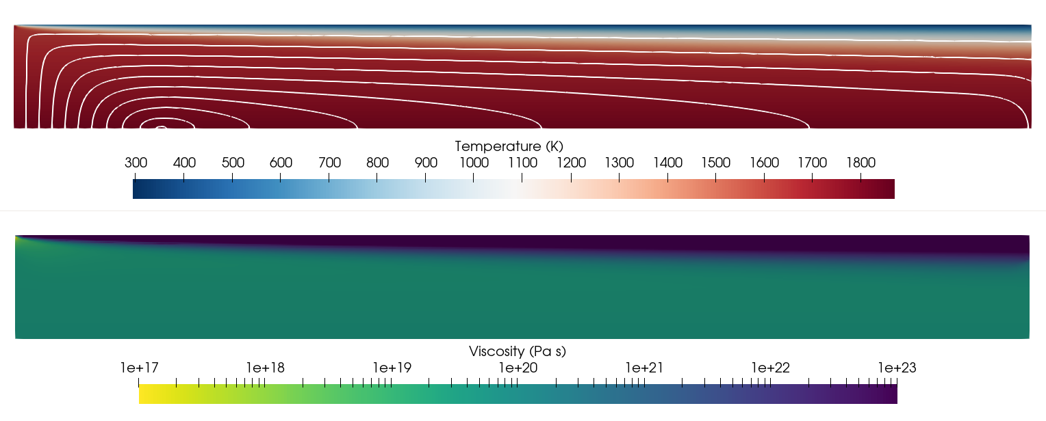
Fig. 118 Setup of cooling oceanic plate model with grain size dependent rheology. Top: Background colors show temperature, streamlines illustrate the flow. Bottom: viscosity.

Grain size evolution.

To model the evolution of the mineral grain size and to take this grain size into account in our rheological model, we use the grain size material model, where these equations are implemented. This model implements a composite diffusion–dislocation rheology, with diffusion creep depending on the evolving grain size, and deformation by dislocation creep reducing the grain size. For more details on this material model and how to use it for global mantle convection models, see Dannberg et al. [2017]. We have to specify the parameters for both creep mechanisms and for the grain size evolution.

subsection Material model
  set Model name = grain size
  subsection Grain size model
    # Diffusion creep has a prefactor, a temperature dependence defined by the
    # activation energy, a pressure dependence defined by the activation volume
    # and a grain size dependence. We take the activation energy from Hirth &
    # Kohlstedt, 2003, and pick the prefactor and activation volume so that we
    # get a reasonable upper mantle viscosity profile and a balance between
    # diffusion and dislocation creep.
    set Diffusion creep prefactor                   = 5e-15
    set Diffusion activation energy                 = 3.75e5
    set Diffusion activation volume                 = 4e-6
    set Diffusion creep grain size exponent         = 3

    # Dislocation creep has a prefactor, a temperature dependence defined by the
    # activation energy, a pressure dependence defined by the activation volume
    # and a strain-rate dependence defined by the exponent. We take the activation
    # energy and volume from Hirth & Kohlstedt, 2003, and pick the prefactor so
    # that we get a reasonable upper mantle viscosity and a balance between
    # diffusion and dislocation creep.
    set Dislocation creep prefactor                 = 1e-15
    set Dislocation activation energy               = 5.3e5
    set Dislocation activation volume               = 1.4e-5
    set Dislocation creep exponent                  = 3.5
    set Dislocation viscosity iteration number      = 10000

    # Grain size is reduced when work is being done by dislocation creep.
    # Here, 10% of this work goes into reducing the grain size rather than
    # into shear heating.
    # Grain size increases with a rate controlled by the grain growth
    # constant and a temperature-depndence defined by the activation
    # energy. By setting the activation volume to zero, we disable the
    # pressure-dependence of grain growth.
    # The parameter values are taken from Dannberg et al., 2017, G-cubed,
    # with the parameters being based on Faul and Jackson, 2007.
    set Work fraction for boundary area change      = 0.1
    set Grain growth rate constant                  = 1.92e-10
    set Grain growth activation energy              = 4e5
    set Grain growth activation volume              = 0

    # Viscosity is cut off at a minimum value of 10^16 Pa s
    # and a maximum value of 10^23 Pa s.
    set Maximum viscosity                           = 1e23
    set Minimum viscosity                           = 1e16
    set Maximum temperature dependence of viscosity = 1e8
  end
end

Many of these parameters, in particular the prefactors and activation volumes, have large uncertainties. The values used here should therefore only be seen as example values. It often makes sense to choose their values based on the viscosity profile one wants to use. These viscosity profiles are usually constrained by observations, such as the geoid or mineral physics data, and therefore provide additional constraints to the values we get from experiments.

Note that diffusion creep depends on the third power of the grain size as specified by the Diffusion creep grain size exponent parameter, and that the stress-dependence of dislocation creep is controlled by the set Dislocation creep exponent parameter.

Tracking the grain size on particles.

To track this evolving mineral grain size on particles, we have to have a compositional field with the name grain_size, we have to specify that we want to advect this field using the particle method, and we have to select grain_size as the particle property to be mapped to this compositional field:

# Our only compositional field is the grain size, and we use particles
# to track it. In order for the grain size to not just be tracked, but
# to evolve over time depending on the temperature and deformation in
# the model, we select ``grain_size'' as the mapped particle property
# for the grain_size compositional field.
subsection Compositional fields
  set Number of fields = 1
  set Names of fields = grain_size
  set Compositional field methods = particles
  set Mapped particle properties = grain_size:grain_size
end

In addition, we have to specify a number of different parameters controlling how to initialize and advect these particles, how to interpolate the computed values back to the mesh and how to control the load balancing. We here choose to add and remove particles in such a way that there are always at least 40 and not more than 640 particles in each cell. This means that a cell with 160 particles can either be refined once (resulting in about 40 particles in each new cell) or coarsened once (resulting in about 640 in the new bigger cell) without having to add or remove particles. We also use the bilinear least squares interpolation scheme to interpolate from the particles to the grid, which is more accurate than schemes based on, for example, the cell average. To make sure this scheme does not generate any over- or under- shoots in the grain size, we switch on the linear least squares limiter. To use this scheme, we also have to update the ghost particles, because the interpolation scheme requires knowledge about particles in neighboring cells. Finally, we use a second Order Runge Kutta integrator to advect the particles.

subsection Postprocess
  set List of postprocessors = visualization, composition statistics, velocity statistics, mass flux statistics, particles

  # We use particles to advect the grain size.
  subsection Particles
    set Interpolation scheme = bilinear least squares
    set Number of particles = 500000
    set Time between data output = 1e6
    set List of particle properties = grain size
    set Load balancing strategy = remove and add particles
    set Minimum particles per cell = 40
    set Maximum particles per cell = 640
    set Integration scheme = rk2
    set Update ghost particles = true

    subsection Interpolator
      subsection Bilinear least squares
        set  Use linear least squares limiter = true
      end
    end
  end
end

Model evolution.

We run the model for 200 million years. In the first few tens of millions of years there are no large changes in the temperature structure, except that the thermal boundary layer increases slightly in thickness. In addition, the grain size evolves from its initially constant value, with the grain size being reduced due to deformation. This leads to a band of particularly low grain size in the lowermost part of the oceanic plate. Grain size is also reduced in the asthenesphere, but to a lesser degree.

At 58.8 Myr, the first downwelling from the base of the lithosphere starts to form. Due to the strong temperature-dependence of the viscosity, only the lowermost part of the plate participates in this downwelling, which is therefore very thin compared to the plate. Because of the strong deformation within the downwelling (which reduces the grain size) and its lower temperature (which hinders grain growth), the grain size in these convective instabilities is smaller compared to the surrounding mantle. Over time, the downwelling moves towards the left and younger plate ages, and additional downwellings start to develop until the model reaches a quasi-steady state.

Fig. 119 Evolution of the temperature (top panels) and grain size (bottom panels) in the model. The first downwelling starts at 58.8 Myr. The full model evolution can be found on YouTube.

Note that for simplicity, our model uses a constant thermal conductivity of 4.7 W/m/K, whereas the thermal conductivity is likely lower in the lithosphere and is also temperature-dependent. Therefore, our lithosphere is thicker (and downwellings occur earlier) than on Earth.