Convection in a 3d box

The world is not two-dimensional. While the previous section introduced a number of the knobs one can play with, things only really become interesting once one goes to 3d. The setup from the previous section is easily adjusted to this and in the following, let us walk through some of the changes we have to consider when going from 2d to 3d. The full input file that contains these modifications and that was used for the simulations we will show subsequently can be found at cookbooks/convection_box_3d.prm.

The first set of changes has to do with the geometry: it is three-dimensional, and we will have to address the fact that a box in 3d has 6 sides, not the 4 we had previously. The documentation of the “box” geometry (see Section Geometry model) states that these sides are numbered as follows: “in 3d, boundary indicators 0 through 5 indicate left, right, front, back, bottom and top boundaries.” Recalling that we want tangential flow all around and want to fix the temperature to known values at the bottom and top, the following will make sense:

set Dimension                              = 3

subsection Geometry model
  set Model name = box

  subsection Box
    set X extent = 1
    set Y extent = 1
    set Z extent = 1
  end
end

subsection Boundary temperature model
  set Fixed temperature boundary indicators   = bottom, top
  set List of model names = box

  subsection Box
    set Bottom temperature = 1
    set Top temperature    = 0
  end
end

subsection Boundary velocity model
  set Tangential velocity boundary indicators = left, right, front, back, bottom, top
end

The next step is to describe the initial conditions. As before, we will use an unstably layered medium but the perturbation now needs to be both in \(x\)- and \(y\)-direction

subsection Initial temperature model
  set Model name = function

  subsection Function
    set Variable names      = x,y,z
    set Function constants  = p=0.01, L=1, pi=3.1415926536, k=1
    set Function expression = (1.0-z) - p*cos(k*pi*x/L)*sin(pi*z)*y^3
  end
end

The third issue we need to address is that we can likely not afford a mesh as fine as in 2d. We choose a mesh that is refined 3 times globally at the beginning, then 3 times adaptively, and is then adapted every 15 time steps. We also allow one additional mesh refinement in the first time step following \(t=0.003\) once the initial instability has given way to a more stable pattern:

subsection Mesh refinement
  set Initial global refinement                = 3
  set Initial adaptive refinement              = 3
  set Time steps between mesh refinement       = 15
  set Additional refinement times              = 0.003
end

Finally, as we have seen in the previous section, a computation with \(Ra=10^4\) does not lead to a simulation that is exactly exciting. Let us choose \(Ra=10^6\) instead (the mesh chosen above with up to 7 refinement levels after some time is fine enough to resolve this). We can achieve this in the same way as in the previous section by choosing \(\alpha=10^{-10}\) and setting

subsection Gravity model
  set Model name = vertical

  subsection Vertical
    set Magnitude = 1e16   # = Ra / Thermal expansion coefficient
  end
end

This has some interesting implications. First, a higher Rayleigh number makes time scales correspondingly smaller; where we generated graphical output only once every 0.01 time units before, we now need to choose the corresponding increment smaller by a factor of 100:

subsection Postprocess
  set List of postprocessors = velocity statistics, temperature statistics, \
                       heat flux statistics, visualization

  subsection Visualization
    set Time between graphical output = 0.0001
  end
end

Secondly, a simulation like this – in 3d, with a significant number of cells, and for a significant number of time steps – will likely take a good amount of time. The computations for which we show results below was run using 64 processors by running it using the command mpirun -n 64 ./aspect convection_box_3d.prm. If the machine should crash during such a run, a significant amount of compute time would be lost if we had to run everything from the start. However, we can avoid this by periodically checkpointing the state of the computation:

subsection Checkpointing
  set Steps between checkpoint = 50
end

If the computation does crash (or if a computation runs out of the time limit imposed by a scheduling system), then it can be restarted from such checkpointing files (see the parameter Resume computation in Section Global parameters).

Running with this input file requires a bit of patience[1] since the number of degrees of freedom is just so large: it starts with a bit over 330,000…

Running with 64 MPI tasks.
Number of active cells: 512 (on 4 levels)
Number of degrees of freedom: 20,381 (14,739+729+4,913)

*** Timestep 0:  t=0 seconds
   Solving temperature system... 0 iterations.
   Rebuilding Stokes preconditioner...
   Solving Stokes system... 18 iterations.

Number of active cells: 1,576 (on 5 levels)
Number of degrees of freedom: 63,391 (45,909+2,179+15,303)

*** Timestep 0:  t=0 seconds
   Solving temperature system... 0 iterations.
   Rebuilding Stokes preconditioner...
   Solving Stokes system... 19 iterations.

Number of active cells: 3,249 (on 5 levels)
Number of degrees of freedom: 122,066 (88,500+4,066+29,500)

*** Timestep 0:  t=0 seconds
   Solving temperature system... 0 iterations.
   Rebuilding Stokes preconditioner...
   Solving Stokes system... 20 iterations.

Number of active cells: 8,968 (on 5 levels)
Number of degrees of freedom: 331,696 (240,624+10,864+80,208)

*** Timestep 0:  t=0 seconds
   Solving temperature system... 0 iterations.
   Rebuilding Stokes preconditioner...
   Solving Stokes system... 21 iterations.
[...]

…but then increases quickly to around 2 million as the solution develops some structure and, after time \(t=0.003\) where we allow for an additional refinement, increases to over 10 million where it then hovers between 8 and 14 million with a maximum of 15,147,534. Clearly, even on a reasonably quick machine, this will take some time: running this on a machine bought in 2011, doing the 10,000 time steps to get to \(t=0.0219\) takes approximately 484,000 seconds (about five and a half days).

The structure or the solution is easiest to grasp by looking at isosurfaces of the temperature. This is shown in Fig. 24 and you can find a movie of the motion that ensues from the heating at the bottom at http://www.youtube.com/watch?v=_bKqU_P4j48. The simulation uses adaptively changing meshes that are fine in rising plumes and sinking blobs and are coarse where nothing much happens. This is most easily seen in the movie at http://www.youtube.com/watch?v=CzCKYyR-cmg. Fig. 25 shows some of these meshes, though still pictures do not do the evolving nature of the mesh much justice. The effect of increasing the Rayleigh number is apparent when comparing the size of features with, for example, the picture at the right of Fig. 18. In contrast to that picture, the simulation is also clearly non-stationary.

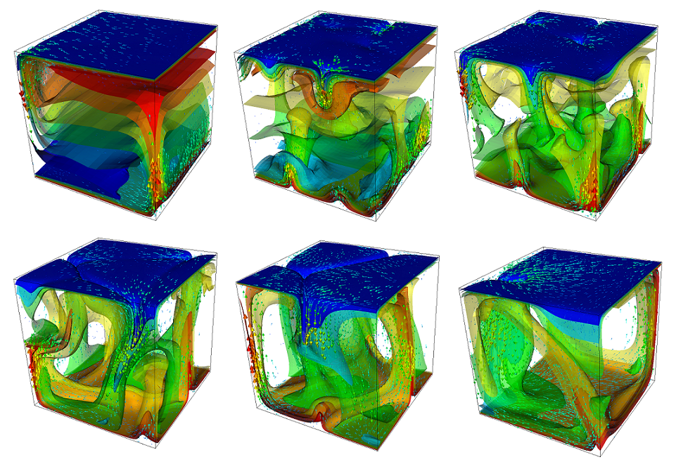
Fig. 24 Convection in a 3d box: Temperature isocontours and some velocity vectors at the first time step after times t=0.001, 0.004, 0.006 (top row, left to right) and t=0.01, 0.013, 0.018 (bottom row).

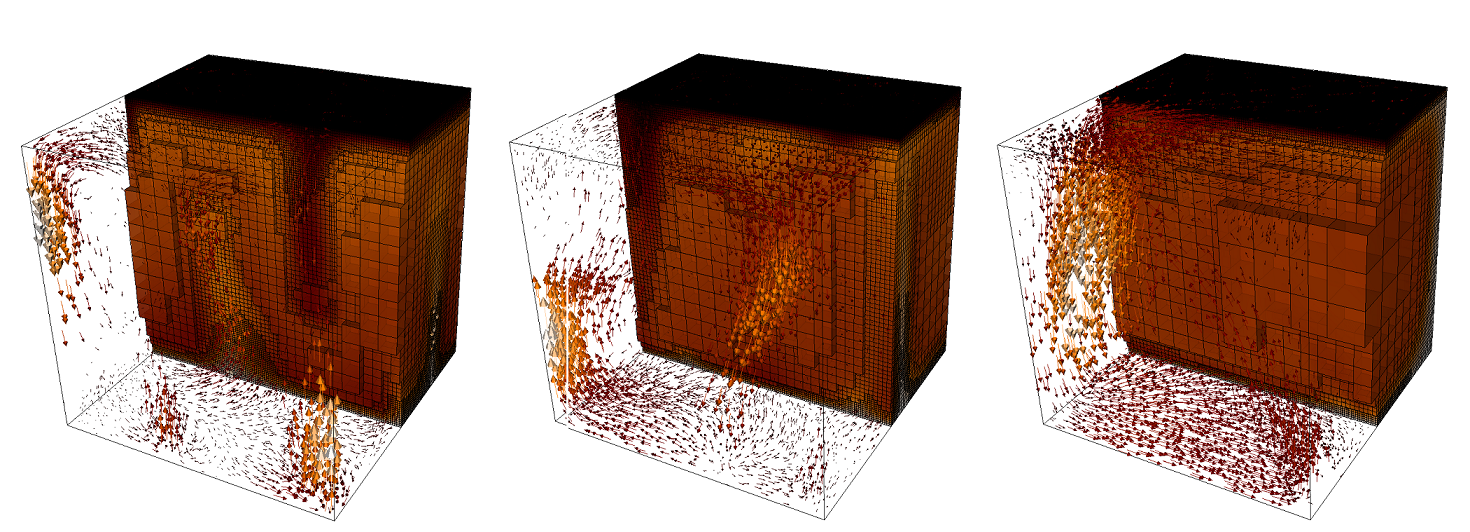
Fig. 25 Convection in a 3d box: Meshes and large-scale velocity field for the third, fourth and sixth of the snapshots shown in Fig. 6.

As before, we could analyze all sorts of data from the statistics file but we will leave this to those interested in specific data. Rather, Fig. 26 only shows the upward heat flux through the bottom and top boundaries of the domain as a function of time.[2] The figure reinforces a pattern that can also be seen by watching the movie of the temperature field referenced above, namely that the simulation can be subdivided into three distinct phases. The first phase corresponds to the initial overturning of the unstable layering of the temperature field and is associated with a large spike in heat flux as well as large velocities (not shown here). The second phase, until approximately \(t=0.01\) corresponds to a relative lull: some plumes rise up, but not very fast because the medium is now stably layered but not fully mixed. This can be seen in the relatively low heat fluxes, but also in the fact that there are almost horizontal temperature isosurfaces in the second of the pictures in Fig. 24. After that, the general structure of the temperature field is that the interior of the domain is well mixed with a mostly constant average temperature and thin thermal boundary layers at the top and bottom from which plumes rise and sink. In this regime, the average heat flux is larger but also more variable depending on the number of plumes currently active. Many other analyses would be possible by using what is in the statistics file or by enabling additional postprocessors.

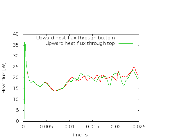
Fig. 26 Convection in a 3d box: Upward heat flux through the bottom and top boundaries as a function of time.

---

[1]

For computations of this size, one should test a few time steps in debug mode but then, of course, switch to running the actual computation in optimized mode – see Section Debug or optimized mode.

[2]

Note that the statistics file actually contains the outward heat flux for each of the six boundaries, which corresponds to the negative of upward flux for the bottom boundary. The figure therefore shows the negative of the values available in the statistics file.