Using the World Builder to model the thermal structure of oceanic transform faults

This section was contributed by Juliane Dannberg.

The input file for this model can be found at cookbooks/transform_fault_behn_2007/transform_fault_behn_2007.prm

Note that this model may take a few hours to run on a laptop because it is a 3D model that runs for a large number of time steps.

This model features the spreading of an oceanic plate away from a mid-ocean ridge, with the ridge axis being segmented by a transform fault. The setup is taken from Behn et al. [2007] and features a box that is 250 km wide, 100 km across, and 100 km in depth. Both oceanic plates move away from the ridge with a velocity of 3 cm/yr, giving a full spreading rate of 6 cm/yr. To achieve this, the velocity is fixed at the top boundary. Material flows in from the bottom, and then leaves the domain at the two sides perpendicular to the spreading direction. The bottom, left and right boundaries are therefore open, prescribing the lithostatic pressure as a boundary condition, whereas the front and back boundaries (parallel to the spreading direction) are (closed) free-slip boundaries. The model ignores buoyancy effects and is therefore fully driven by the boundary conditions. The initial temperature follows a half-space cooling model for each of the two ridge segments, created by the Geodynamic World Builder. Adiabatic heating and shear heating are not enabled. The figure below shows the initial temperature distribution.

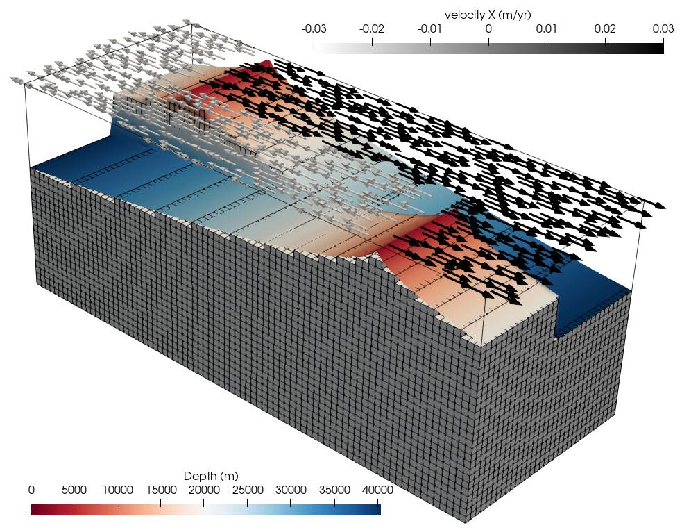
Fig. 120 Setup of the transform fault model. Background colors show depth of the 1500 K isotherm, arrows illustrate the velocity. The mesh is shown in the bottom part of the model.

Creating the initial temperature with the Geodynamic World Builder

The initial thermal structure of the model should follow a half-space cooling model for each of the two ridge segments. The easiest way of creating this temperature distribution is to use the Geodynamic World Builder, which allows us to define features such as oceanic plates together with the desired thermal structure. Since the Geodynamic World Builder is included in the ASPECT installation, we only need to create an input file for the World Builder and then our thermal structure will be generated as part of the model run. For details on how to create this Geodynamic World Builder input file, see the corresponding tutorial in the Geodynamic World Builder manual.

In the .prm file for ASPECT, we just have to make sure that we set this file as the World builder file, that we use `world builder’ as our initial temperature models and that our material properties are consistent between the two files. Specifically, we here want to make sure that the surface temperature and the adiabatic/mantle potential temperature are the same.

# We use the Geodynamic World Builder to create the initial temperature.
# Therefore, we have to specify the location of the GWB input file
# that we want to use. The file we use here is located in the cookbooks
# folder of the GWB repository. See the corresponding tutorial in the
# Geodynamic World Builder on how to create this file.
set World builder file = $ASPECT_SOURCE_DIR/contrib/world_builder/cookbooks/3d_cartesian_transform_fault/3d_cartesian_transform_fault.wb

# Note that the adiabatic surface temperature should be consistent with the
# value assumed in the GWB input file, given in the parameter 'potential
# mantle temperature'.
set Adiabatic surface temperature          = 1573.15

# The initial temperature comes form the Geodynamic World Builder.
subsection Initial temperature model
  set List of model names = world builder
end

# We prescribe the surface temperature at the top and the mantle potential temperature
# at the bottom.
subsection Boundary temperature model
  set Fixed temperature boundary indicators   = top, bottom

  set List of model names = box
  subsection Box
    set Top temperature = 273.15
    set Bottom temperature = 1573.15
  end
end

Since the thermal structure is computed according to the half-space cooling model, we also need to ensure that we use the same thermal diffusivity as in the Geodynamic World Builder input file:

subsection Material model
  set Model name = visco plastic

  subsection Visco Plastic
    set Reference temperature = 1573.15
    set Heat capacities       = 1000
    set Densities             = 3300           # Value from Behn et al., 2007
    set Thermal expansivities = 0              # Thermal buoyancy is ignored in Behn et al., 2007

    set Define thermal conductivities = true
    set Thermal conductivities        = 3.5
  end
end

Note that the thermal expansivity is set to zero because thermal buoyancy is ignored in Behn et al. [2007].

We here present two cases following Behn et al. [2007]: Case 1, which has a constant viscosity, and case 2, which has a temperature-dependent viscosity. The full input files can be found at cookbooks/transform_fault_behn_2007/transform_fault_behn_2007.prm and

cookbooks/transform_fault_behn_2007/temperature_dependent.prm.

Thermal structure at the end of the model run.

We run the models for 10 million years and then evaluate the thermal structure. Specifically, we here show a comparison to Figures 3 and 4 in Behn et al. [2007].

Fig. 121 Thermal structure at 20 km depth for the initial state (top), the final state of the model with constant viscosity (middle) and the model with a temperature-dependent viscosity (bottom). Gray line indicates the location of the plate boundary. Arrows illustrate the flow field.

Fig. 122 Thermal structure in a vertical slice through the center of the transform fault at the final state of the model with constant viscosity (top) and the model with a temperature-dependent viscosity (bottom). Left column shows the strain rate, right column shows the temperature distribution. Black arrows illustrate the flow field.

The temperature-dependent viscosity reduces the temperature and focuses the upwelling below the transform fault, leading to more deformation in that region.