Reading in compositional initial composition files generated with geomIO#
This section was contributed by Juliane Dannberg
Note
This cookbook is based on a developer version of geomIO from July 2016. In the meantime, the development of geomIO continued, and there is now a publication [Bauville and Baumann, 2019] that describes its features and how they can be used in more detail.
Many geophysical setups require initial conditions with several different materials and complex geometries. Hence, sometimes it would be easier to generate the initial geometries of the materials as a drawing instead of by writing code. The MATLAB-based library geomIO (https://bitbucket.org/geomio/geomio, [Bauville and Baumann, 2019] provides a convenient tool to convert a drawing generated with the vector graphics editor Inkscape (https://inkscape.org/en/) to a data file that can be read into ASPECT. Here, we will demonstrate how this can be done for a 2D setup for a model with one compositional field, but geomIO also has the capability to create 3D volumes based on a series of 2D vector drawings using any number of different materials. Similarly, initial conditions defined in this way can also be used with particles instead of compositional fields.
To obtain the developer version of geomIO, you can clone the bitbucket repository by executing the command
git clone https://bitbucket.org/geomio/geomio.git
or you can download geomIO here.
You will then need to add the geomIO
source folders to your MATLAB path by running the file located in
/path/to/geomio/installation/InstallGeomIO.m. An extensive documentation for
how to use geomIO can be found here. Among other things, it explains how
to generate drawings in Inkscape that can be read in by geomIO, which
involves assigning new attributes to paths in Inkscape’s XML editor. In
particular, a new property ‘phase’ has to be added to each path,
and set to a value corresponding to the index of the material that should be
present in this region in the initial condition of the geodynamic model.
Note
geomIO currently only supports the latest stable version of Inkscape (0.91), and
other versions might not work with geomIO or cause errors. Moreover, geomIO
currently does not support grouping paths (paths can still be combined using Path\(\rightarrow\)Union,Path\(\rightarrow\)Difference or similar commands),
and only the outermost closed contour of a path will be considered. This means
that, for example, for modeling a spherical annulus, you would have to draw two
circles, and assign the inner one the same phase as the background of your
drawing.
We will here use a drawing of a jellyfish located in cookbooks/geomio/doc/jellyfish.svg, where different phases have already been assigned to each path (Fig. 65).

Fig. 65 Vector drawing of a jellyfish.#
Note
The page of your drawing in Inkscape should already have the extents (in px) that you later want to use in your model (in m).
After geomIO is initialized in MATLAB, we run geomIO as described in the documentation, loading the default options and then specifying all the option we want to change, such as the path to the input file, or the resolution:
% set options for geomIO
opt                 = geomIO_Options();
opt.inputFileName   = ['/path/to/aspect/doc/manual/cookbooks/geomio/jellyfish.svg'];
opt.DrawCoordRes    = 21; % optionally change resolution with opt.DrawCoordRes = your value;

% run geomIO
[PathCoord]         = run_geomIO(opt,'2D');
You can view all of the options available by typing opt in MATLAB.
In the next step we create the grid that is used for the coordinates in the
ascii data initial conditions file and assign a phase to each grid point:
% define the bounding box for the output mesh
% (this should be the X extent and Y extent in your ASPECT model)
xmin = 0; xmax = opt.svg.width;
ymin = 0; ymax = opt.svg.height;

% set the resolution in the output file:
% [Xp,Yp] = ndgrid(xmin:your_steplength_x:xmax,ymin:your_steplength_y:ymax);
[Xp,Yp]      = ndgrid(xmin:15:xmax,ymin:15:ymax);
Phase        = zeros(size(Xp));

% assign a phase to each grid point according to your drawing
Phase = assignPhase2Markers(PathCoord, opt, Xp, Yp, Phase);

% plot your output
figure(2)
scatter(Xp(:),Yp(:),10,Phase(:),'filled');
axis equal
axis([xmin xmax ymin ymax])
You can plot the Phase variable in MATLAB to see if the drawing was read in
and all phases are assigned correctly (Fig. 66).
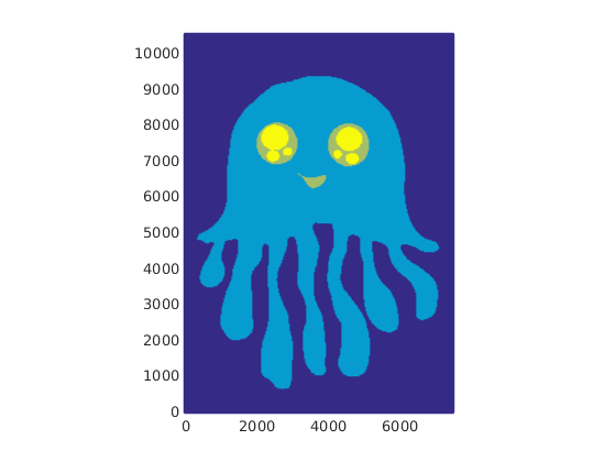
Fig. 66 Plot of the Phase variable in MATLAB.#
Finally, we want to write output in a format that can be read in by ASPECT’s
ascii data compositional initial conditions plugin. We write the data into
the file jelly.txt:
% the headers ASPECT needs for the ascii data plugin
header1 = 'x';
header2 = 'y';
header3 = 'phase';

% create an array in the correct format for the ascii data plugin
Vx = Xp(:);
Vy = Yp(:);
VPhase = Phase(:);
[m,n] = size(Phase);

% write the data into the output file
fid=fopen('jelly.txt','w');
fprintf(fid, '# POINTS: %d %d \n',[m n]);
fprintf(fid, ['# Columns: ' header1 ' ' header2 ' ' header3 '\n']);
fprintf(fid, '%f %f %f \n', [Vx Vy VPhase]');
fclose(fid);
To read in the file we just created (a copy is located in ASPECT’s data
directory), we set up a model with a box geometry with the same extents we
specified for the drawing in px and one compositional field. We choose the
ascii data compositional initial conditions and specify that we want to read
in our jellyfish. The relevant parts of the input file are listed below:
subsection Geometry model
  set Model name = box

  # The extents of the box is the same as the width
  # and height of the drawing in px
  # (an A4 page = 7350x10500 px).
  subsection Box
    set X extent = 7350
    set Y extent = 10500
  end
end

# We need one compositional field that will be assigned
# the values read in from the ascii data plugin.
subsection Compositional fields
  set Number of fields = 1
end

# We use the ascii data plugin to read in the file created with geomIO.
subsection Initial composition model
  set Model name = ascii data

  subsection Ascii data model
    set Data directory       = $ASPECT_SOURCE_DIR/data/initial-composition/ascii-data/test/
    set Data file name       = jelly.txt
  end
end

# We refine the mesh where compositional gradients are
# high, i.e. at the boundary between the different phases
# assigned to the compositional field through the initial
# condition.
subsection Mesh refinement
  set Refinement fraction                      = 0.99
  set Coarsening fraction                      = 0
  set Initial global refinement                = 5
  set Initial adaptive refinement              = 4
  set Time steps between mesh refinement       = 0
  set Strategy                                 = composition
end
If we look at the output in ParaView, we can see our jellyfish, with the
mesh refined at the boundaries between the different phases
(Fig. 67).

Fig. 67 ASPECT model output of the jellyfish and corresponding mesh in ParaView.#
For a geophysical setup, the MATLAB code could be extended to write out the
phases into several different columns of the ASCII data file (corresponding to
different compositional fields). This initial conditions file could then be
used in ASPECT with a material model such as the multicomponent model, assigning
each phase different material properties.
An animation of a model using the jellyfish as initial condition and assigning it a higher viscosity can be found here: https://www.youtube.com/watch?v=YzNTubNG83Q.