The SolCx Stokes benchmark#

The SolCx benchmark is intended to test the accuracy of the solution to a problem that has a large jump in the viscosity along a line through the domain. Such situations are common in geophysics: for example, the viscosity in a cold, subducting slab is much larger than in the surrounding, relatively hot mantle material.

The SolCx benchmark computes the Stokes flow field of a fluid driven by spatial density variations, subject to a spatially variable viscosity. Specifically, the domain is \(\Omega=[0,1]^2\), gravity is \(\mathbf g=(0,-1)^T\) and the density is given by \(\rho(\mathbf x)=\sin(\pi x_1)\cos(\pi x_2)\); this can be considered a density perturbation to a constant background density. The viscosity is

\[\begin{split}\begin{aligned} \eta(\mathbf x) = \left\{ \begin{matrix} 1 & \text{for}\ x_1 \le 0.5, \\ 10^6 & \text{for}\ x_1 > 0.5. \end{matrix} \right.\end{aligned}\end{split}\]

This strongly discontinuous viscosity field yields an almost stagnant flow in the right half of the domain and consequently a singularity in the pressure along the interface. Boundary conditions are free slip on all of \(\partial\Omega\). The temperature plays no role in this benchmark. The prescribed density field and the resulting velocity field are shown in Fig. 177 and Fig. 178.

The SolCx benchmark was previously used in Section 4.1.1 of Duretz et al. [2011] (references to earlier uses of the benchmark are available there) and its analytic solution is given in Zhong [1996]. ASPECT contains an implementation of this analytic solution taken from the Underworld package (see Moresi et al. [2007] and http://www.underworldproject.org/, and correcting for the mismatch in sign between the implementation and the description in Duretz et al. [2011]).

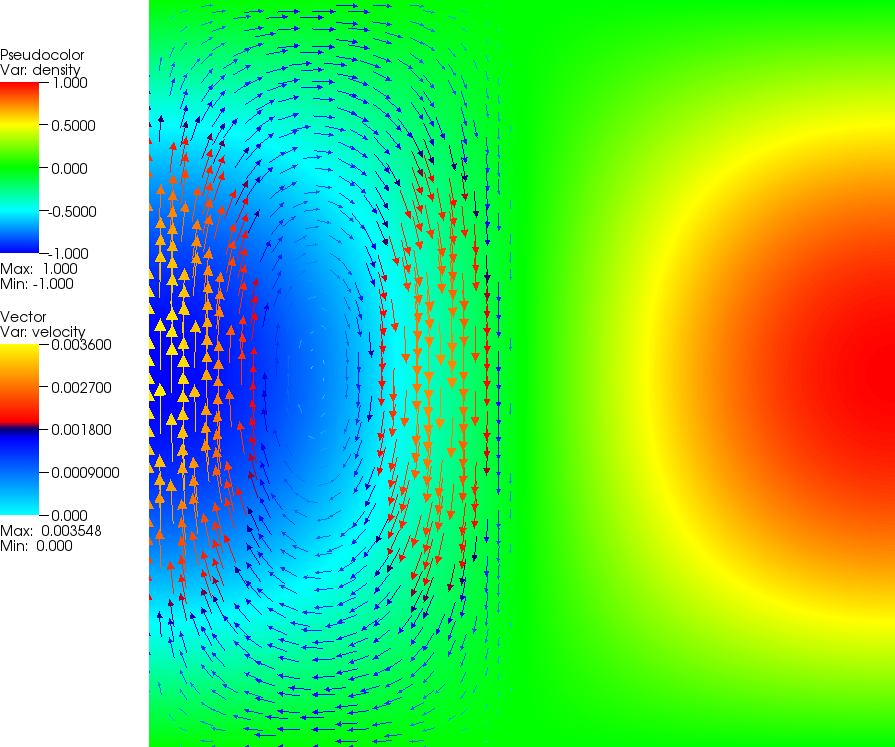
Fig. 177 SolCx Stokes benchmark. The density perturbation field and overlaid to it some velocity vectors. The viscosity is very large in the right hand, leading to a stagnant flow in this region.#

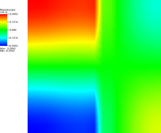
Fig. 178 SolCx Stokes benchmark. The pressure on a relatively coarse mesh, showing the internal layer along the line where the viscosity jumps.#

To run this benchmark, the following input file will do (see the files in benchmarks/solcx/ to rerun the benchmark):

set Additional shared libraries            = ./libsolcx.so

############### Global parameters

set Dimension                              = 2
set Start time                             = 0
set End time                               = 0
set Output directory                       = output
set Pressure normalization                 = volume

############### Parameters describing the model

subsection Geometry model
  set Model name = box

  subsection Box
    set X extent = 1
    set Y extent = 1
  end
end

subsection Boundary velocity model
  set Tangential velocity boundary indicators = left, right, bottom, top
end

subsection Material model
  set Model name = SolCxMaterial

  subsection SolCx
    set Viscosity jump = 1e6
  end
end

subsection Gravity model
  set Model name = vertical
end

############### Parameters describing the temperature field

subsection Initial temperature model
  set Model name = perturbed box
end

############### Parameters describing the discretization

subsection Discretization
  set Stokes velocity polynomial degree       = 2
  set Use locally conservative discretization = false
end

subsection Mesh refinement
  set Initial adaptive refinement              = 0
  set Initial global refinement                = 4
end

############### Parameters describing what to do with the solution

subsection Postprocess
  set List of postprocessors = SolCxPostprocessor, visualization
end

Since this is the first cookbook in the benchmarking section, let us go through the different parts of this file in more detail:

The material model and the postprocessor
The first part consists of parameter setting for overall parameters. Specifically, we set the dimension in which this benchmark runs to two and choose an output directory. Since we are not interested in a time dependent solution, we set the end time equal to the start time, which results in only a single time step being computed.

The last parameter of this section, Pressure normalization, is set in such a way that the pressure is chosen so that its domain average is zero, rather than the pressure along the surface, see Section Pressure normalization.
The next part of the input file describes the setup of the benchmark. Specifically, we have to say how the geometry should look like (a box of size \(1\times 1\)) and what the velocity boundary conditions shall be (tangential flow all around - the box geometry defines four boundary indicators for the left, right, bottom and top boundaries, see also Geometry model). This is followed by subsections choosing the material model (where we choose a particular model implemented in that describes the spatially variable density and viscosity fields, along with the size of the viscosity jump) and finally the chosen gravity model (a gravity field that is the constant vector \((0,-1)^T\), see Gravity model).
The part that follows this describes the boundary and initial values for the temperature. While we are not interested in the evolution of the temperature field in this benchmark, we nevertheless need to set something. The values given here are the minimal set of inputs.
The second-to-last part sets discretization parameters. Specifically, it determines what kind of Stokes element to choose (see Discretization and the extensive discussion in Kronbichler et al. [2012]). We do not adaptively refine the mesh but only do four global refinement steps at the very beginning. This is obviously a parameter worth playing with.
The final section on postprocessors determines what to do with the solution once computed. Here, we do two things: we ask to compute the error in the solution using the setup described in Duretz et al. [2011], and we request that output files for later visualization are generated and placed in the output directory. The functions that compute the error automatically query which kind of material model had been chosen, i.e., they can know whether we are solving the SolCx benchmark or one of the other benchmarks discussed in the following subsections.

Upon running with this input file, you will get output of the following kind (obviously with different timings, and details of the output may also change as development of the code continues):

aspect/cookbooks> ../aspect solcx.prm
Number of active cells: 256 (on 5 levels)
Number of degrees of freedom: 3,556 (2,178+289+1,089)

*** Timestep 0:  t=0 years
   Solving temperature system... 0 iterations.
   Rebuilding Stokes preconditioner...
   Solving Stokes system... 30+3 iterations.

   Postprocessing:
     Errors u_L1, p_L1, u_L2, p_L2: 1.125997e-06, 2.994143e-03, 1.670009e-06, 9.778441e-03
     Writing graphical output:      output/solution/solution-00000



+---------------------------------------------+------------+------------+
| Total wallclock time elapsed since start    |      1.51s |            |
|                                             |            |            |
| Section                         | no. calls |  wall time | % of total |
+---------------------------------+-----------+------------+------------+
| Assemble Stokes system          |         1 |     0.114s |       7.6% |
| Assemble temperature system     |         1 |     0.284s |        19% |
| Build Stokes preconditioner     |         1 |    0.0935s |       6.2% |
| Build temperature preconditioner|         1 |    0.0043s |      0.29% |
| Solve Stokes system             |         1 |    0.0717s |       4.8% |
| Solve temperature system        |         1 |  0.000753s |      0.05% |
| Postprocessing                  |         1 |     0.627s |        42% |
| Setup dof systems               |         1 |      0.19s |        13% |
+---------------------------------+-----------+------------+------------+

One can then visualize the solution in a number of different ways (see Section Visualizing results), yielding pictures like those shown in Fig. 177 and Fig. 178. One can also analyze the error as shown in various different ways, for example as a function of the mesh refinement level, the element chosen, etc.; we have done so extensively in Kronbichler et al. [2012].