Crustal deformation#
This section was contributed by Cedric Thieulot, and makes use of the Drucker-Prager material model written by Anne Glerum and the free surface plugin by Ian Rose.
This is a simple example of an upper-crust undergoing compression or extension. It is characterized by a single layer of visco-plastic material subjected to basal kinematic boundary conditions. In compression, this setup is somewhat analogous to Willett [1999], and in extension to Allken et al. [2011].
Brittle failure is approximated by adapting the viscosity to limit the stress
that is generated during deformation. This “cap” on the stress
level is parameterized in this experiment by the pressure-dependent Drucker
Prager yield criterion and we therefore make use of the Drucker-Prager
material model (see Material model) in the
cookbooks/crustal_deformation/crustal_model_2D.prm.
The layer is assumed to have dimensions of \(80\text{ km} \times 16\text{ km}\) and to have a density \(\rho=2800\text{ kg/m}^3\). The plasticity parameters are specified as follows:
subsection Material model
  set Model name = drucker prager

  subsection Drucker Prager
    set Reference density = 2800

    subsection Viscosity
      set Minimum viscosity = 1e19
      set Maximum viscosity = 1e25
      set Reference strain rate = 1e-20
      set Angle internal friction = 30
      set Cohesion = 20e6
    end
  end
end
The yield strength \(\sigma_y\) is a function of pressure, cohesion and angle of friction (see Drucker-Prager material model in Section Material model), and the effective viscosity is then computed as follows:
where \(\dot{\epsilon}\) is the square root of the second invariant of the deviatoric strain rate. The viscosity cutoffs ensure that the viscosity remains within computationally acceptable values.
During the first iteration of the first timestep, the strain rate is zero, so
we avoid dividing by zero by setting the strain rate to
Reference strain rate.
The top boundary is a free surface while the left, right and bottom boundaries are subjected to the following boundary conditions:
subsection Boundary velocity model
  subsection Function
    set Variable names      = x,y
    set Function constants  = cm=0.01, year=1
    set Function expression =  if (x<40e3 , 1*cm/year, -1*cm/year) ; 0
  end
end
Note that compressive boundary conditions are simply achieved by reversing the sign of the imposed velocity.
The free surface will be advected up and down according to the solution of the Stokes solve. We have a choice whether to advect the free surface in the direction of the surface normal or in the direction of the local vertical (i.e., in the direction of gravity). For small deformations, these directions are almost the same, but in this example the deformations are quite large. We have found that when the deformation is large, advecting the surface vertically results in a better behaved mesh, so we set the following in the free surface subsection:
subsection Free surface
  set Surface velocity projection = vertical
end
We also make use of the strain rate-based mesh refinement plugin:
subsection Mesh refinement
  set Initial adaptive refinement        = 1
  set Initial global refinement          = 3
  set Refinement fraction                = 0.95
  set Strategy                           = strain rate
  set Coarsening fraction                = 0.05
  set Time steps between mesh refinement = 1
  set Run postprocessors on initial refinement = true
end
Setting set Initial adaptive refinement = 4 yields a series of meshes as
shown in Fig. 98, all produced during the first timestep. As expected, we
see that the location of the highest mesh refinement corresponds to the
location of a set of conjugated shear bands.
If we now set this parameter to 1 and allow the simulation to evolve for 500kyr, a central graben or plateau (depending on the nature of the boundary conditions) develops and deepens/thickens over time, nicely showcasing the unique capabilities of the code to handle free surface large deformation, localised strain rates through visco-plasticity and adaptive mesh refinement as shown in Fig. 99.
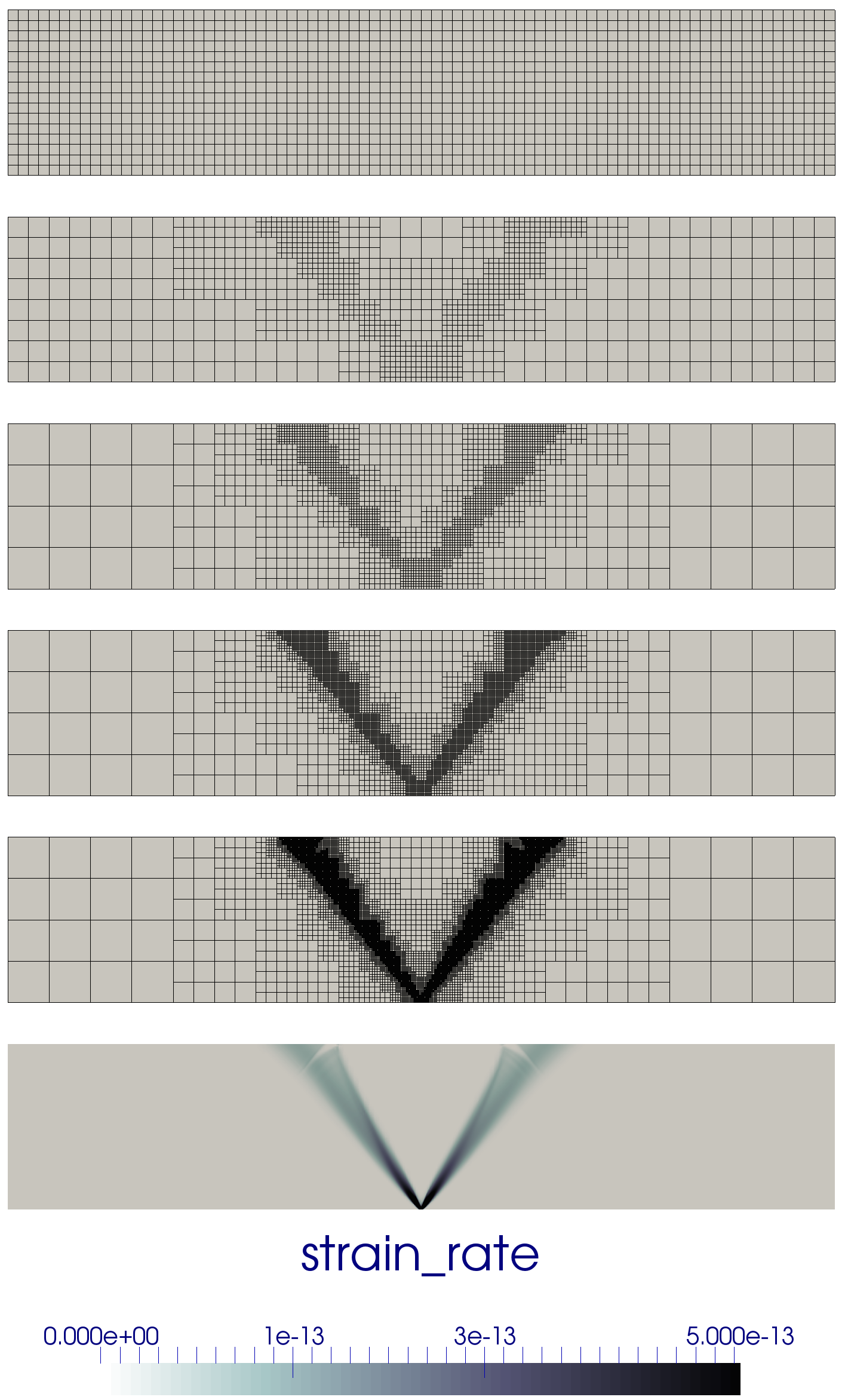
Fig. 98 Mesh evolution during the first timestep (refinement is based on strain rate).#
Deformation localizes at the basal velocity discontinuity and plastic shear bands form at an angle of approximately \(53^\circ\) to the bottom in extension and \(35^\circ\) in compression, both of which correspond to the reported Arthur angle [Buiter, 2012, Kaus, 2010].
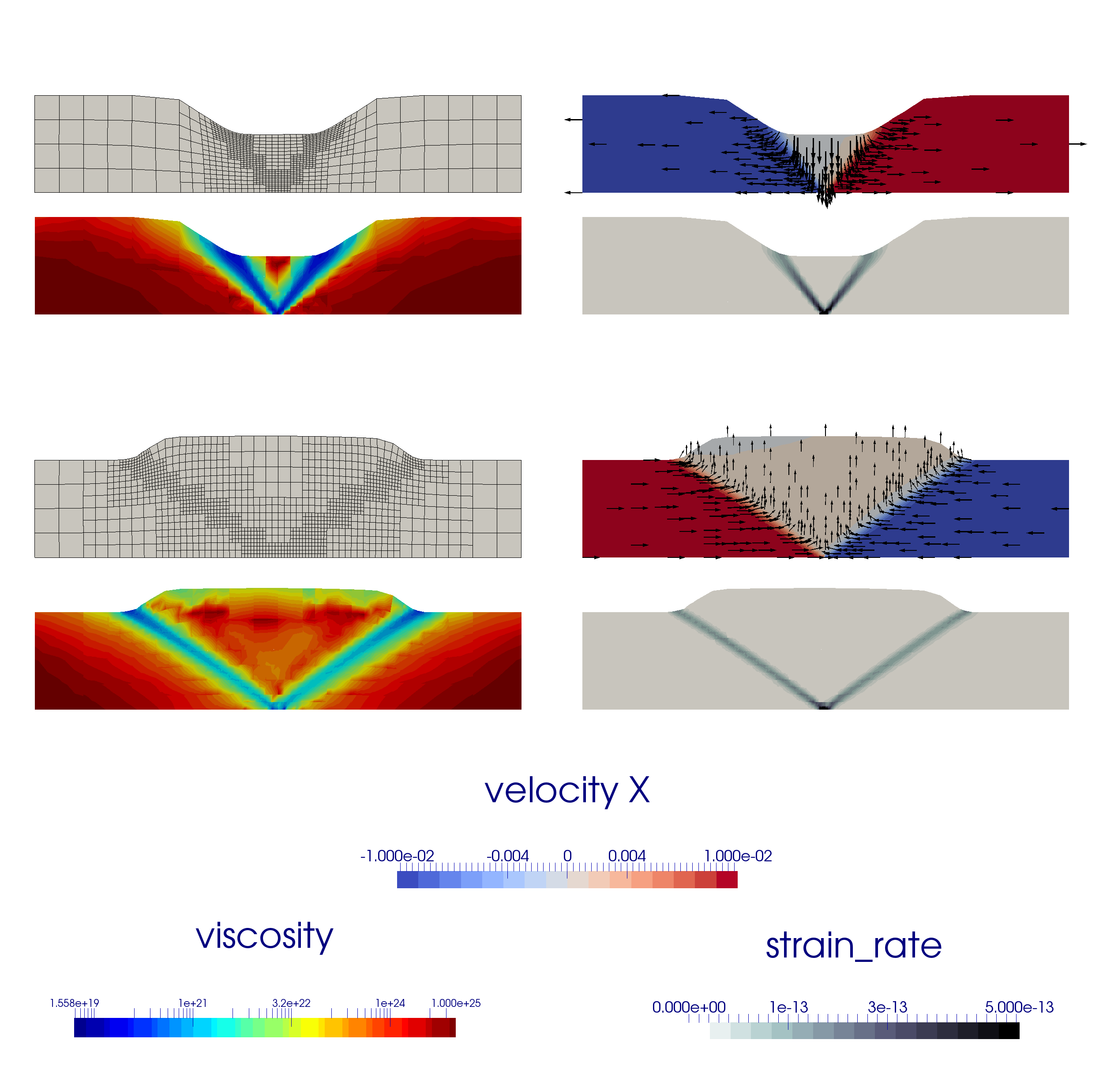
Fig. 99 Finite element mesh, velocity, viscosity and strain rate fields in the case of extensional boundary conditions (top) and compressive boundary conditions (bottom) at t=500kyr.#
Extension to 3D#
We can easily modify the previous input file to produce crustal_model_3D.prm
which implements a similar setup, with the additional constraint that the
position of the velocity discontinuity varies with the \(y\)-coordinate, as
shown in Fig. 100. The domain is now \(128\times96\times16\) km and the
boundary conditions are implemented as follows:
subsection Boundary velocity model
  subsection Function
    set Variable names      = x,y,z
    set Function constants  = cm=0.01, year=1
    set Function expression =  if (x<56e3 && y<=48e3 | x<72e3 && y>48e3,-1*cm/year,1*cm/year);0;0
  end
end
The presence of an offset between the two velocity discontinuity zones leads to a transform fault which connects them.
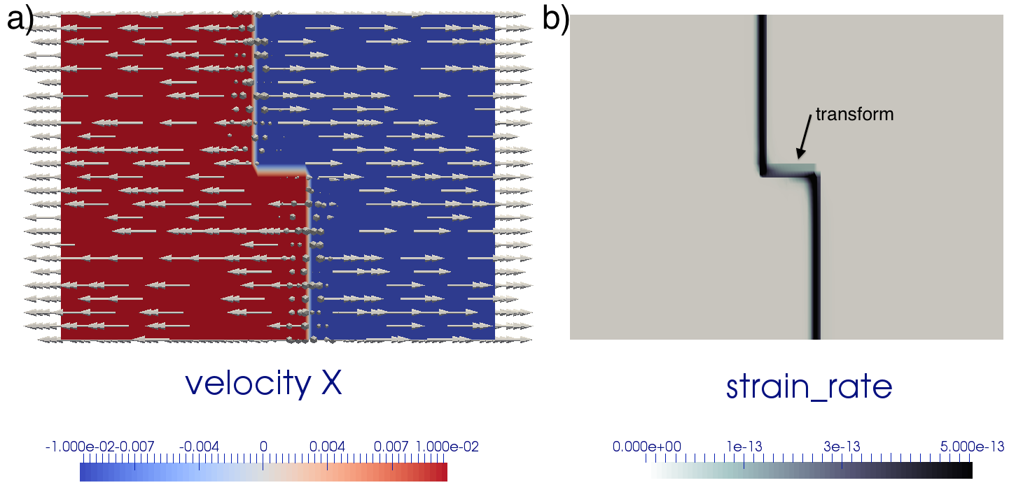
Fig. 100 Basal velocity boundary conditions and corresponding strain rate field for the 3D model.#
The Finite Element mesh, the velocity, viscosity and strain rate fields are shown in Fig. 101 at the end of the first time steps. The reader is encouraged to run this setup in time to look at how the two grabens interact as a function of their initial offset [Allken et al., 2011, Allken et al., 2012, Allken et al., 2013].
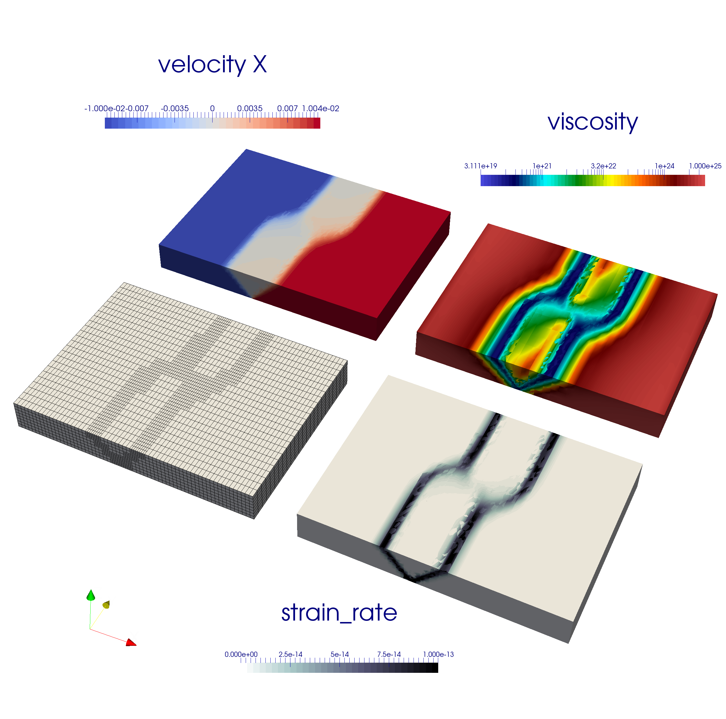
Fig. 101 Finite element mesh, velocity, viscosity and strain rate fields at the end of the first time step after one level of strain rate-based adaptive mesh refinement.#