Simple convection in a spherical 3d shell

The setup from the previous section can of course be extended to 3d shell geometries as well – though at significant computational cost. In fact, the number of modifications necessary is relatively small, as we will discuss below. To show an example up front, a picture of the temperature field one gets from such a simulation is shown in Fig. 81. The corresponding movie can be found at http://youtu.be/j63MkEc0RRw.

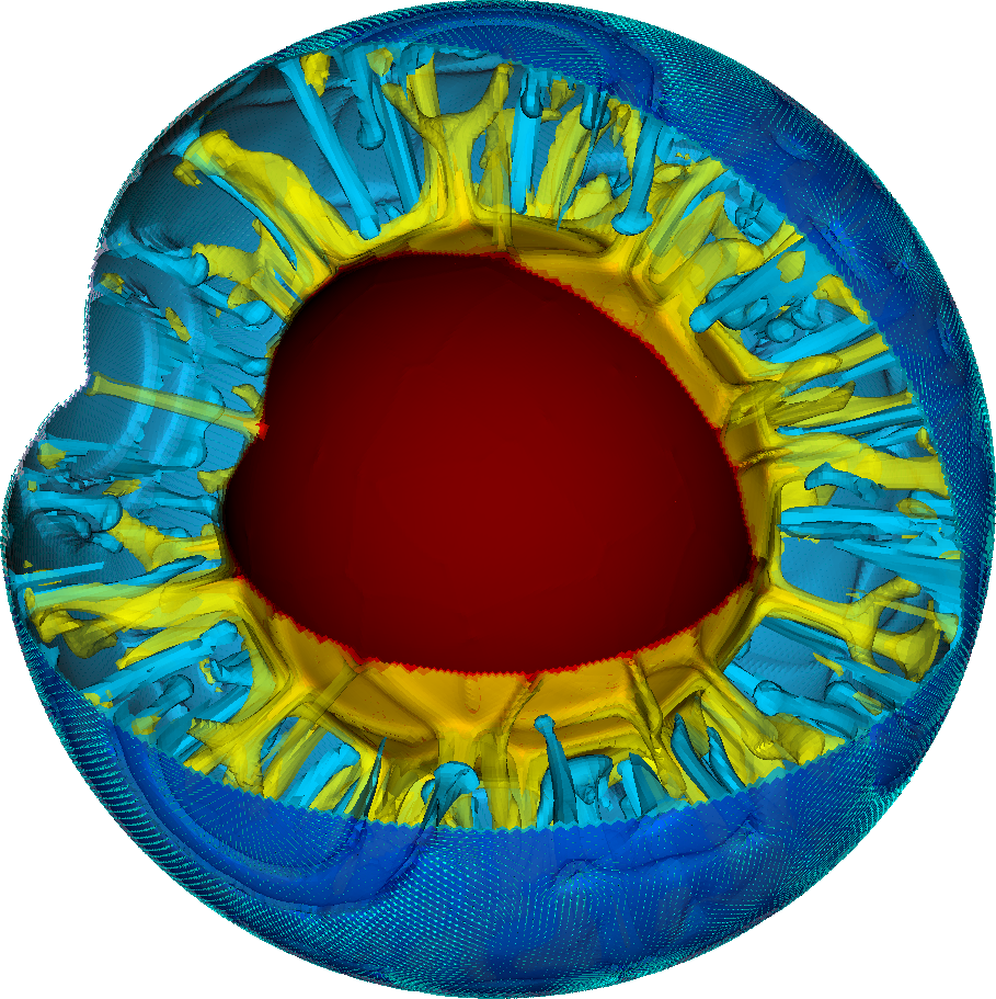
Fig. 81 Convection in a spherical shell: Snapshot of isosurfaces of the temperature field at time \(t\approx 1.06\times10^{9}\) years with a quarter of the geometry cut away. The surface shows vectors indicating the flow velocity and direction.

The input file.

Compared to the input file discussed in the previous section, the number of changes is relatively small. However, when taking into account the various discussions about which parts of the model were or were not realistic, they go throughout the input file, so we reproduce it here in its entirety, interspersed with comments (the full input file can also be found in cookbooks/shell_simple_3d/shell_simple_3d.prm). Let us start from the top where everything looks the same except that we set the dimension to 3:

set Dimension                              = 3
set Use years in output instead of seconds = true
set End time                               = 1.5e9
set Output directory                       = output-shell_simple_3d

subsection Material model
  set Model name = simple

  subsection Simple model
    set Thermal expansion coefficient = 4e-5
    set Viscosity                     = 1e22
  end
end

The next section concerns the geometry. The geometry model remains unchanged at “spherical shell” but we omit the opening angle of 90 degrees as we would like to get a complete spherical shell. Such a shell of course also only has two boundaries (the inner one has indicator zero, the outer one indicator one) and consequently these are the only ones we need to list in the “Boundary velocity model” section:

subsection Geometry model
  set Model name = spherical shell

  subsection Spherical shell
    set Inner radius  = 3481000
    set Outer radius  = 6336000
  end
end

subsection Boundary velocity model
  set Zero velocity boundary indicators       = inner
  set Tangential velocity boundary indicators = outer
end

Next, since we convinced ourselves that the temperature range from 973 to 4273 was too large given that we do not take into account adiabatic effects in this model, we reduce the temperature at the inner edge of the mantle to 1973. One can think of this as an approximation to the real temperature there minus the amount of adiabatic heating material would experience as it is transported from the surface to the core-mantle boundary. This is, in effect, the temperature difference that drives the convection (because a completely adiabatic temperature profile is stable despite the fact that it is much hotter at the core mantle boundary than at the surface). What the real value for this temperature difference is, is unclear from current research, but it is thought to be around 1000 Kelvin, so let us choose these values.

subsection Boundary temperature model
  set Fixed temperature boundary indicators = inner, outer
  set List of model names = spherical constant

  subsection Spherical constant
    set Inner temperature = 1973
    set Outer temperature = 973
  end
end

The second component to this is that we found that without adiabatic effects, an initial temperature profile that decreases the temperature from the inner to the outer boundary makes no sense. Rather, we expected a more or less constant temperature with boundary layers at both ends. We could describe such an initial temperature field, but since any initial temperature is mostly arbitrary anyway, we opt to just assume a constant temperature in the middle between the inner and outer temperature boundary values and let the simulation find the exact shape of the boundary layers itself:

subsection Initial temperature model
  set Model name = function

  subsection Function
    set Function expression = 1473
  end
end

subsection Gravity model
  set Model name = ascii data
end

As before, we need to determine how many mesh refinement steps we want. In 3d, it is simply not possible to have as much mesh refinement as in 2d, so we choose the following values that lead to meshes that have, after an initial transitory phase, between 1.5 and 2.2 million cells and 50–75 million unknowns:

subsection Mesh refinement
  set Initial global refinement          = 2
  set Initial adaptive refinement        = 3
  set Strategy                           = temperature
  set Time steps between mesh refinement = 15
end

Second to last, we specify what we want ASPECT to do with the solutions it computes. Here, we compute the same statistics as before, and we again generate graphical output every million years. Computations of this size typically run with  1000 MPI processes, and it is not efficient to let every one of them write their own file to disk every time we generate graphical output; rather, we group all of these into a single file to keep file systems reasonably happy. Likewise, to accommodate the large amount of data, we output depth averaged fields in VTU format since it is easier to visualize:

subsection Postprocess
  set List of postprocessors = visualization, velocity statistics, \
                temperature statistics, heat flux statistics, \
          depth average

  subsection Visualization
    set Output format                 = vtu
    set Time between graphical output = 1e6
    set Number of grouped files       = 1
  end

  subsection Depth average
    set Time between graphical output = 1.5e6
    set Output format                 = vtu
  end
end

Finally, we realize that when we run very large parallel computations, nodes go down or the scheduler aborts programs because they ran out of time. With computations this big, we cannot afford to just lose the results, so we checkpoint the computations every 50 time steps and can then resume it at the last saved state if necessary (see Section Checkpoint/restart support):

subsection Checkpointing
  set Steps between checkpoint = 50
end

Evaluation.

Just as in the 2d case above, there are still many things that are wrong from a physical perspective in this setup, notably the no-slip boundary conditions at the bottom and of course the simplistic material model with its fixed viscosity and its neglect for adiabatic heating and compressibility. But there are also a number of things that are already order of magnitude correct here.

For example, if we look at the heat flux this model produces, we find that the convection here produces approximately the correct number. Wikipedia’s article on Earth’s internal heat budget[1] states that the overall heat flux through the Earth surface is about \(47\times10^{12}\) W (i.e., 47 terawatts) of which an estimated 12–30 TW are primordial heat released from cooling the Earth and 15–41 TW from radiogenic heating.[2] Our model does not include radiogenic heating (though ASPECT has a number of Heating models to switch this on, see Heating model) but we can compare what the model gives us in terms of heat flux through the inner and outer boundaries of our shell geometry. This is shown in Fig. 82 where we plot the heat flux through boundaries zero and one, corresponding to the core-mantle boundary and Earth’s surface. ASPECT always computes heat fluxes in outward direction, so the flux through boundary zero will be negative, indicating the we have a net flux into the mantle as expected. The figure indicates that after some initial jitters, heat flux from the core to the mantle stabilizes at around 4.5 TW and that through the surface at around 10 TW, the difference of 5.5 TW resulting from the overall cooling of the mantle. While we cannot expect our model to be quantitatively correct, this can be compared with estimated heat fluxes of 5–15 TW for the core-mantle boundary, and an estimated heat loss due to cooling of the mantle of 7–15 TW (values again taken from Wikipedia).

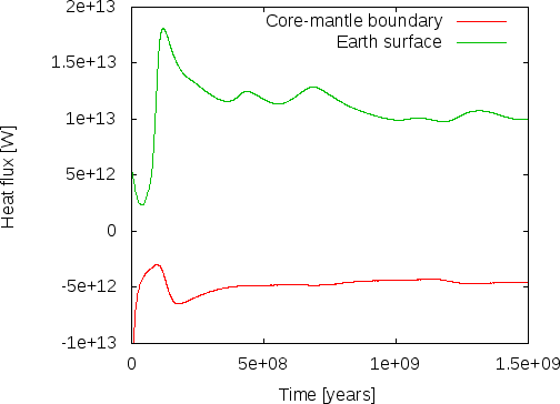
Fig. 82 Evaluating the 3d spherical shell model. Outward heat fluxes through the inner and outer boundaries of the shell.

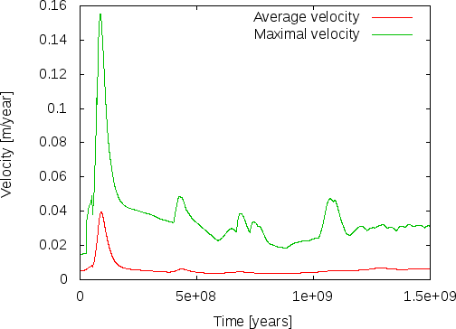
Fig. 83 Evaluating the 3d spherical shell model. Average and maximal velocities in the mantle.

A second measure of whether these results make sense is to compare velocities in the mantle with what is known from observations. As shown in Fig. 83, the maximal velocities settle to values on the order of 3 cm/year (each of the peaks in the line for the maximal velocity corresponds to a particularly large plume rising or falling). This is, again, at least not very far from what we know to be correct and we should expect that with a more elaborate material model we should be able to get even closer to reality.

---

[1]

Not necessarily the most scientific source, but easily accessible and typically about right in terms of numbers. The numbers stated here are those listed on Wikipedia at the time this section was written in March 2014.

[2]

As a point of reference, for the mantle an often used number for the release of heat due to radioactive decay is \(7.4\times 10^{-12}\) W/kg. Taking a density of \(3300\; \text{ kg}/\text{m}^3\) and a volume of \(10^{12}\; \text{ m}^3\) would yield roughly \(2.4\times 10^{13}\) W of heat produced. This back of the envelope calculation lies within the uncertain range stated above.