The passive case.

We will consider the exact same situation as in the previous section but we will ask where the material that started in the bottom 20% of the domain ends up, as well as the material that started in the top 20%. For the moment, let us assume that there is no material between the materials at the bottom, the top, and the middle. The way to describe this situation is to simply add the following block of definitions to the parameter file (you can find the full parameter file in cookbooks/composition_passive/composition_passive.prm:

# This is the new part: We declare that there will
# be two compositional fields that will be
# advected along. Their initial conditions are given by
# a function that is one for the lowermost 0.2 height
# units of the domain and zero otherwise in the first case,
# and one in the top most 0.2 height units in the latter.
subsection Compositional fields
  set Number of fields = 2
end

subsection Initial composition model
  set Model name = function

  subsection Function
    set Variable names      = x,y
    set Function expression = if(y<0.2, 1, 0) ; if(y>0.8, 1, 0)
  end
end

Running this simulation yields results such as the ones shown in Fig. 28 – Fig. 33 where we show the values of the functions \(c_1(\mathbf x,t)\) and \(c_2(\mathbf x,t)\) at various times in the simulation. Because these fields were one only inside the lowermost and uppermost parts of the domain, zero everywhere else, and because they have simply been advected along with the flow field, the places where they are larger than one half indicate where material has been transported to so far.1

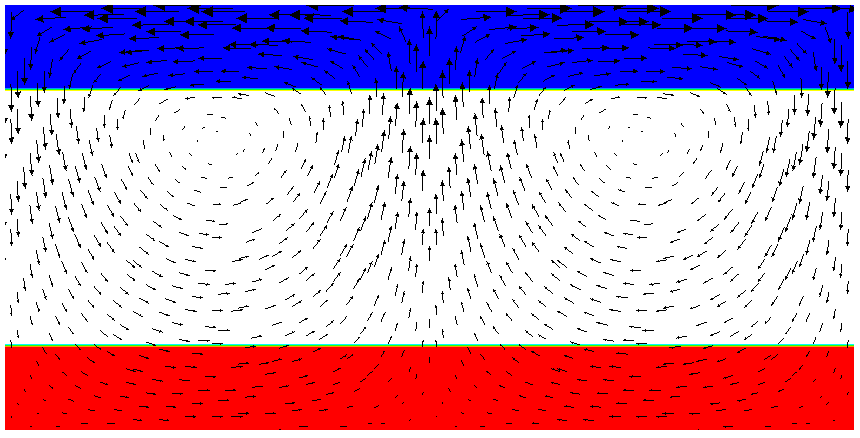
Fig. 28 Passive compositional fields: The figures show, at different times in the simulation, the velocity field along with those locations where the first compositional field is larger than 0.5 (in red, indicating the locations where material from the bottom of the domain has gone) as well as where the second compositional field is larger than 0.5 (in blue, indicating material from the top of the domain. The results were obtained with two more global refinement steps compared to the cookbooks/composition_passive/composition_passive.prm input file.

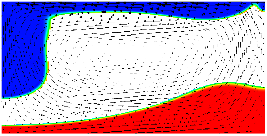
Fig. 29 Passive compositional fields: The figures show, at different times in the simulation, the velocity field along with those locations where the first compositional field is larger than 0.5 (in red, indicating the locations where material from the bottom of the domain has gone) as well as where the second compositional field is larger than 0.5 (in blue, indicating material from the top of the domain. The results were obtained with two more global refinement steps compared to the cookbooks/composition_passive/composition_passive.prm input file.

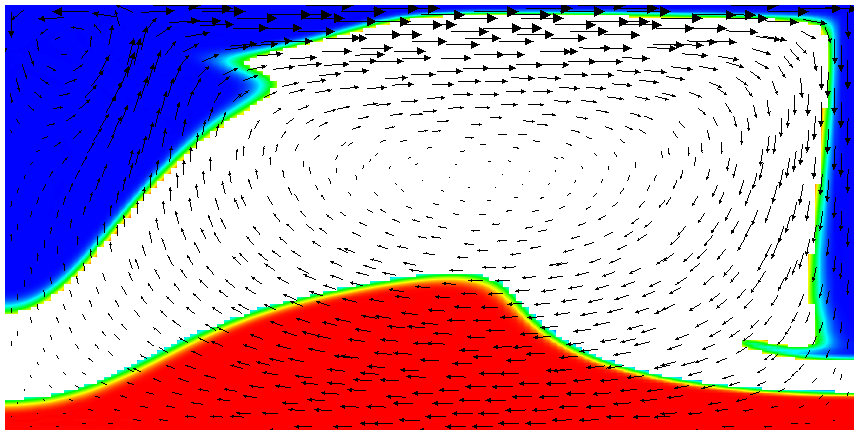
Fig. 30 Passive compositional fields: The figures show, at different times in the simulation, the velocity field along with those locations where the first compositional field is larger than 0.5 (in red, indicating the locations where material from the bottom of the domain has gone) as well as where the second compositional field is larger than 0.5 (in blue, indicating material from the top of the domain. The results were obtained with two more global refinement steps compared to the cookbooks/composition_passive/composition_passive.prm input file.

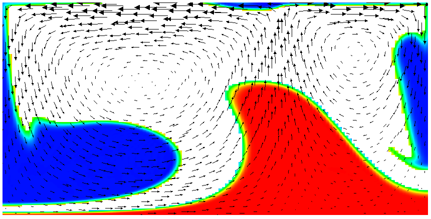
Fig. 31 Passive compositional fields: The figures show, at different times in the simulation, the velocity field along with those locations where the first compositional field is larger than 0.5 (in red, indicating the locations where material from the bottom of the domain has gone) as well as where the second compositional field is larger than 0.5 (in blue, indicating material from the top of the domain. The results were obtained with two more global refinement steps compared to the cookbooks/composition_passive/composition_passive.prm input file.

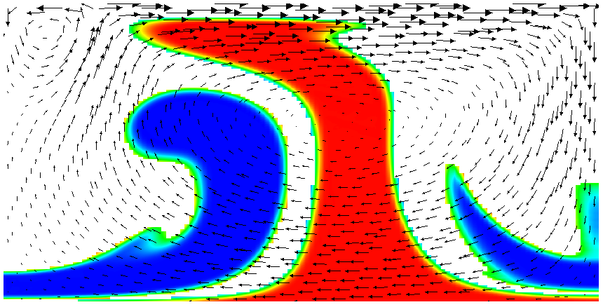
Fig. 32 Passive compositional fields: The figures show, at different times in the simulation, the velocity field along with those locations where the first compositional field is larger than 0.5 (in red, indicating the locations where material from the bottom of the domain has gone) as well as where the second compositional field is larger than 0.5 (in blue, indicating material from the top of the domain. The results were obtained with two more global refinement steps compared to the cookbooks/composition_passive/composition_passive.prm input file.

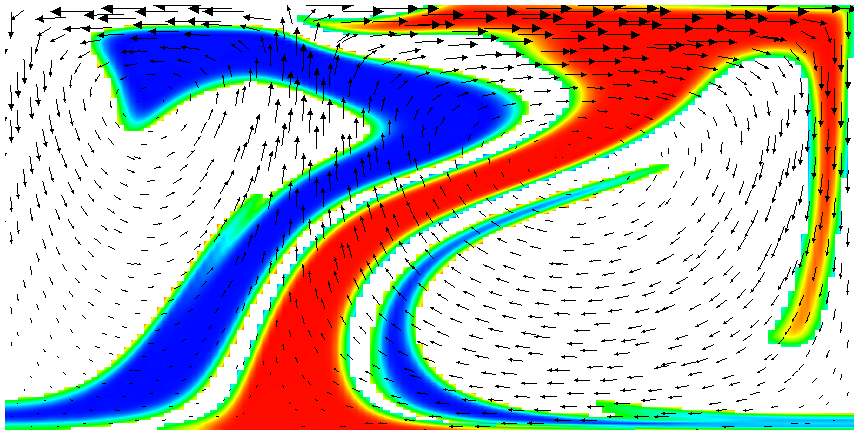
Fig. 33 Passive compositional fields: The figures show, at different times in the simulation, the velocity field along with those locations where the first compositional field is larger than 0.5 (in red, indicating the locations where material from the bottom of the domain has gone) as well as where the second compositional field is larger than 0.5 (in blue, indicating material from the top of the domain. The results were obtained with two more global refinement steps compared to the cookbooks/composition_passive/composition_passive.prm input file.

Fig. 33 shows one aspect of compositional fields that occasionally makes them difficult to use for very long time computations. The simulation shown here runs for 20 time units, where every cycle of the spreading center at the top moving left and right takes 4 time units, for a total of 5 such cycles. While this is certainly no short-term simulation, it is obviously visible in the figure that the interface between the materials has diffused over time.

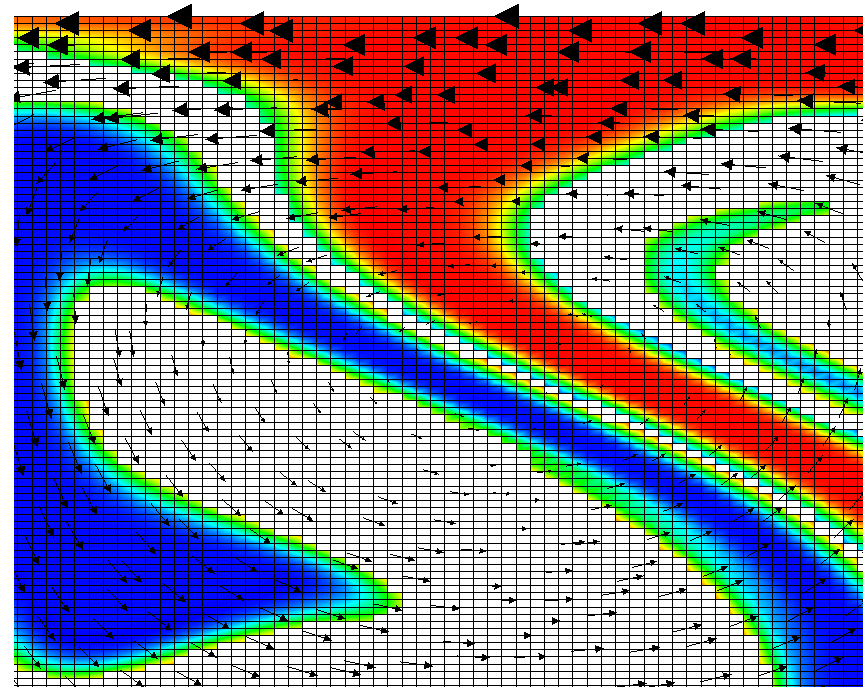
Fig. 34 Passive compositional fields: A later image of the simulation corresponding to the sequence shown above and zoom-in on the center, also showing the mesh.

Fig. 34 shows a zoom into the center of the domain at the final time of the simulation. The figure only shows values that are larger than 0.5, and it looks like the transition from red or blue to the edge of the shown region is no wider than 3 cells. This means that the computation is not overly diffusive but it is nevertheless true that this method has difficulty following long and thin filaments2. This is an area in which may see improvements in the future.

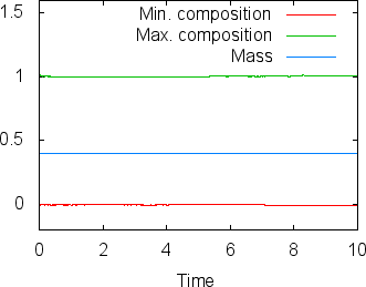
Fig. 35 Passive compositional fields: Minimum and maximum of the first compositional variable over time, as well as the mass \(m_1(t)=\int_\Omega c_1(\mathbf x,t)\) stored in this variable.

A different way of looking at the quality of compositional fields as opposed to particles is to ask whether they conserve mass. In the current context, the mass contained in the \(i\)th compositional field is \(m_i(t)=\int_\Omega c_i(\mathbf x,t)\). This can easily be achieve in the following way, by adding the composition statistics postprocessor:

subsection Postprocess
  set List of postprocessors = visualization, temperature statistics, composition statistics
end

While the scheme we use to advect the compositional fields is not strictly conservative, it is almost perfectly so in practice. For example, in the computations shown in this section (using two additional global mesh refinements over the settings in the parameter file cookbooks/composition_passive/composition_passive.prm), Fig. 35 shows the maximal and minimal values of the first compositional fields over time, along with the mass \(m_1(t)\) (these are all tabulated in columns of the statistics file, see Overview and Visualizing statistical data). While the maximum and minimum fluctuate slightly due to the instability of the finite element method in resolving discontinuous functions, the mass appears stable at a value of 0.403646 (the exact value, namely the area that was initially filled by each material, is 0.4; the difference is a result of the fact that we can’t exactly represent the step function on our mesh with the finite element space). In fact, the maximal difference in this value between time steps 1 and 500 is only \(1.1\times 10^{-6}\). In other words, these numbers show that the compositional field approach is almost exactly mass conservative.

---

1

Of course, this interpretation suggests that we could have achieved the same goal by encoding everything into a single function – that would, for example, have had initial values one, zero and minus one in the three parts of the domain we are interested in.

2

We note that this is no different for particles where the position of particles has to be integrated over time and is subject to numerical error. In simulations, their location is therefore not the exact one but also subject to a diffusive process resulting from numerical inaccuracies. Furthermore, in long thin filaments, the number of particles per cell often becomes too small and new particles have to be inserted; their properties are then interpolated from the surrounding particles, a process that also incurs a smoothing penalty.