2D compressible convection with a reference profile and material properties from BurnMan

This section was contributed by Juliane Dannberg and René Gassmöller

In this cookbook we will set up a compressible mantle convection model that uses the (truncated) anelastic liquid approximation (see The anelastic liquid approximation (ALA) and The truncated anelastic liquid approximation (TALA)), together with a reference profile read in from an ASCII data file. The data we use here is generated with the open source mineral physics toolkit BurnMan (https://geodynamics.github.io/burnman/) using the python example program simple_adiabat.py. This file is available as a part of BurnMan, and provides a tutorial for how to generate ASCII data files that can be used together with ASPECT. The computation is based on the Birch-Murnaghan equation of state, and uses a harzburgitic composition. However, in principle, other compositions or equations of state can be used, as long as the reference profile contains data for the reference temperature, pressure, density, gravity, thermal expansivity, specific heat capacity and compressibility. Using BurnMan to generate the reference profile has the advantage that all the material property data are consistent, for example, the gravity profile is computed using the reference density.

Fig. 88 Reference profile generated using Burnman.

The reference profile is shown in Fig. 88, and the corresponding data file is located at data/adiabatic-conditions/ascii-data/isentrope_properties.txt.

Setting up the ASPECT model

In order to use this profile, we have to import and use the data in the adiabatic conditions model, in the gravity model and in the material model, which is done using the corresponding ASCII data plugins. The input file is provided in cookbooks/burnman/burnman.prm, and it uses the 2d shell geometry previously discussed in Simple convection in a quarter of a 2d annulus and surface velocities imported from GPlates as explained in Using reconstructed surface velocities by GPlates.

To use the BurnMan data in the material model, we have to specify that we want to use the ascii reference profile model. This material model makes use of the functionality provided by the AsciiData classes in ASPECT, which allow plugins such as material models, boundary or initial conditions models to read in ASCII data files (see for example Reading in compositional initial composition files generated with geomIO). Hence, we have to provide the directory and file name of the data to be used in the separate subsection Ascii data model, and the same functionality and syntax will also be used for the adiabatic conditions and gravity model.

The viscosity in this model is computed as the product of a profile \(\eta_r(z)\), where \(z\) corresponds to the depth direction of the chosen geometry model, and a term that describes the dependence on temperature:

\[\begin{aligned} \eta(z,T) = \eta_r(z) \eta_0 \exp\left(-A \frac{T - T_{\text{adi}}}{T_{\text{adi}}}\right), \end{aligned}\]

where \(A\) and \(\eta_0\) are constants determined in the input file via the parameters Viscosity and Thermal viscosity exponent, and \(\eta_r(z)\) is a stepwise constant function that determines the viscosity profile. This function can be specified by providing a list of Viscosity prefactors and a list of depths that describe in which depth range each prefactor should be applied, in other words, at which depth the viscosity changes. By default, it is set to viscosity jumps at 150 km depth, between upper mantle and transition zone, and between transition zone and lower mantle). The prefactors used here lead to a low-viscosity asthenosphere, and high viscosities in the lower mantle. To make sure that these viscosity jumps do not lead to numerical problems in our computation (see Averaging material properties), we also use harmonic averaging of the material properties.

subsection Material model
  set Model name = ascii reference profile

  subsection Ascii data model
    set Data file name = isentrope_properties.txt
    set Data directory = $ASPECT_SOURCE_DIR/data/adiabatic-conditions/ascii-data/
  end

  subsection Ascii reference profile
    set Thermal viscosity exponent = 10.0
    set Viscosity prefactors = 1.0, 0.1, 1.0, 10.0
  end

  set Material averaging = harmonic average
end

As the reference profile has a depth dependent density and also contains data for the compressibility, this material model supports compressible convection models.

For the adiabatic conditions and the gravity model, we also specify that we want to use the respective ascii data plugin, and provide the data directory in the same way as for the material model. The gravity model automatically uses the same file as the adiabatic conditions model.

subsection Adiabatic conditions model
  set Model name = ascii data

  subsection Ascii data model
    set Data directory = $ASPECT_SOURCE_DIR/data/adiabatic-conditions/ascii-data/
    set Data file name = isentrope_properties.txt
  end
end

subsection Gravity model
  set Model name = ascii data
end

To make use of the reference state we just imported from BurnMan, we choose a formulation of the equations that employs a reference state and compressible convection, in this case the anelastic liquid approximation (see The anelastic liquid approximation (ALA)).

subsection Formulation
  set Formulation = anelastic liquid approximation
end

This means that the reference profiles are used for all material properties in the model, except for the density in the buoyancy term (on the right-hand side of the force balance equation (1), which in the limit of the anelastic liquid approximation becomes Equation (20)). In addition, the density derivative in the mass conservation equation (see Mass conservation approximation) is taken from the adiabatic conditions, where it is computed as the depth derivative of the provided reference density profile (see also Combined formulations).

Visualizing the model output

If we look at the output of our model (for example in ParaView), we can see how cold, highly viscous slabs are subducted and hot plumes rise from the core-mantle boundary. The final time step of the model is shown in Fig. 89, and the full model evolution can be found at https://youtu.be/nRBOpw5kp-4. Visualizing material properties such as density, thermal expansivity or specific heat shows how they change with depth, and reveals abrupt jumps at the phase transitions, where properties change from one mineral phase to the next. We can also visualize the gravity and the adiabatic profile, to ensure that the data we provided in the data/adiabatic-conditions/ascii-data/isentrope_properties.txt file is used in our model.

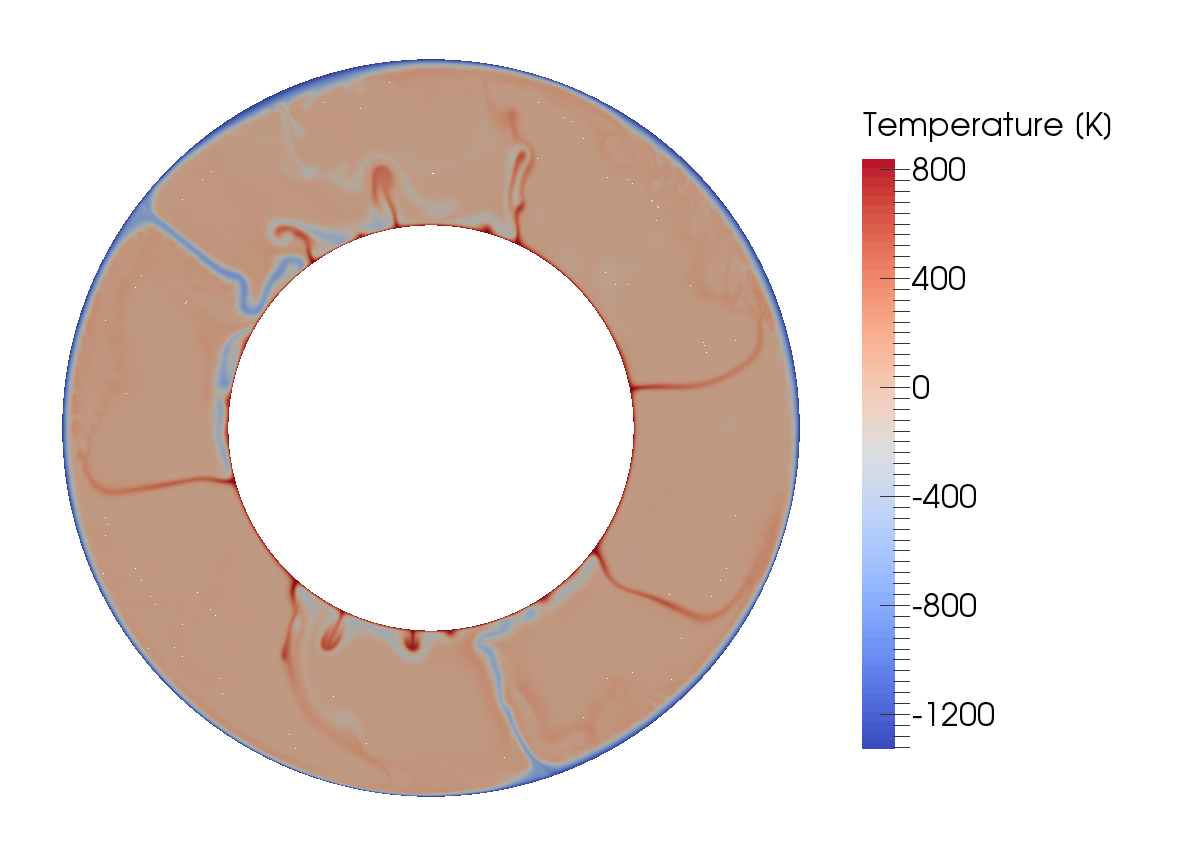
Fig. 89 Compressible convection in a 2d spherical shell, using a reference profile exported form BurnMan, which is based on the Birch-Murnaghan equation of state. The figure shows the state at the end of the model evolution over 260 Ma.

Comparing different model approximations

For the model described above, we have used the anelastic liquid approximation. However, one might want to use different approximations that employ a reference state, such as the truncated anelastic liquid approximation (TALA, see The truncated anelastic liquid approximation (TALA)), which is also supported by the ascii reference profile material model. In this case, the only change compared to ALA is in the density used in the buoyancy term, the only place where the temperature-dependent density instead of the reference density is used. For the TALA, this density only depends on the temperature (and not on the dynamic pressure, as in the ALA). Hence, we have to make this change in the appropriate place in the material model (while keeping the formulation of the equations set to anelastic liquid approximation):

subsection Material model
  subsection Ascii reference profile
    set Use TALA = true
  end
end

We now want to compare these commonly used approximations to the “isothermal compression approximation” (see The isothermal/isentropic compression approximation (ICA)) that is unique to ASPECT. It does not require a reference state and uses the full density everywhere in the equations except for the right-hand side mass conservation, where the compressibility is used to compute the density derivative with regard to pressure. Nevertheless, this formulation can make use of the reference profile computed by BurnMan and compute the dependence of material properties on temperature and pressure in addition to that by taking into account deviations from the reference profile in both temperature and pressure. As this requires a modification of the equations outside of the material model, we have to specify this change in the Formulation (and remove the lines for the use of TALA discussed above).

subsection Formulation
  set Formulation = isentropic compression
end

As the “isothermal compression approximation” is also ASPECT’s default for compressible models, the same model setup can also be achieved by just removing the lines that specify which Formulation should be used.

Fig. 90 and Fig. 91 show a comparison between the different models. They demonstrate that upwellings and downwellings may occur in slightly different places and at slightly different times when using a different approximation, but averaged model properties describing the state of the model – such as the root mean square velocity – are similar between the models.

Fig. 90 Comparison between the anelastic liquid approximation, the truncated anelastic liquid approximation and the isothermal compression approximation, showing the temperature distribution for the different models at the end of the model evolution at 260 Ma.

Fig. 91 Comparison between the anelastic liquid approximation, the truncated anelastic liquid approximation and the isothermal compression approximation, showing the evolution of the root mean square velocity.