The active case.

The next step, of course, is to make the flow actually depend on the composition. After all, compositional fields are not only intended to indicate where material come from, but also to indicate the properties of this material. In general, the way to achieve this is to write material models where the density, viscosity, and other parameters depend on the composition, taking into account what the compositional fields actually denote (e.g., if they simply indicate the origin of material, or the concentration of things like olivine, perovskite, …). The construction of material models is discussed in much greater detail in Section Material models; we do not want to revisit this issue here and instead choose – once again – the simplest material model that is implemented in the Subsection: Material model / Simple model.

The place where we are going to hook in a compositional dependence is the density. In the simple model, the density is fundamentally described by a material that expands linearly with the temperature; for small density variations, this corresponds to a density model of the form \(\rho(T)=\rho_0(1-\alpha(T-T_0))\). This is, by virtue of its simplicity, the most often considered density model. But the simple model also has a hook to make the density depend on the first compositional field \(c_1(\mathbf x,t)\), yielding a dependence of the form \(\rho(T)=\rho_0(1-\alpha(T-T_0))+\gamma c_1\). Here, let us choose \(\rho_0=1, \alpha=0.01, T_0=0, \gamma=100\). The rest of our model setup will be as in the passive case above. Because the temperature will be between zero and one, the temperature induced density variations will be restricted to 0.01, whereas the density variation by origin of the material is 100. This should make sure that dense material remains at the bottom despite the fact that it is hotter than the surrounding material.1

This setup of the problem can be described using an input file that is almost completely unchanged from the passive case. The only difference is the use of the following section (the complete input file can be found in cookbooks/composition_active/composition_active.prm:

subsection Material model
  set Model name = simple

  subsection Simple model
    set Thermal conductivity                           = 1e-6
    set Thermal expansion coefficient                  = 0.01
    set Viscosity                                      = 1
    set Reference density                              = 1
    set Reference temperature                          = 0
    set Density differential for compositional field 1 = 0.1
  end
end

To debug the model, we will also want to visualize the density in our graphical output files. This is done using the following addition to the postprocessing section, using the density visualization plugin:

subsection Postprocess
  set List of postprocessors = visualization, temperature statistics, composition statistics

  subsection Visualization
    set List of output variables = density
    set Time between graphical output = 0.1
  end
end

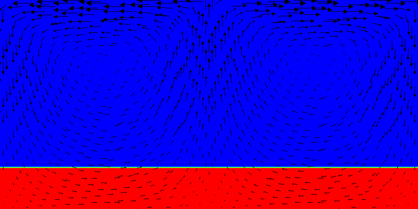
Fig. 36 Active compositional fields: Compositional field 1 at the time t=0. Compared to the results shown in Fig. 33 it is clear that the heavy material stays at the bottom of the domain now. The effect of the density on the velocity field is also clearly visible by noting that at all three times the spreading center at the top boundary is in exactly the same position; this would result in exactly the same velocity field if the density and temperature were constant.

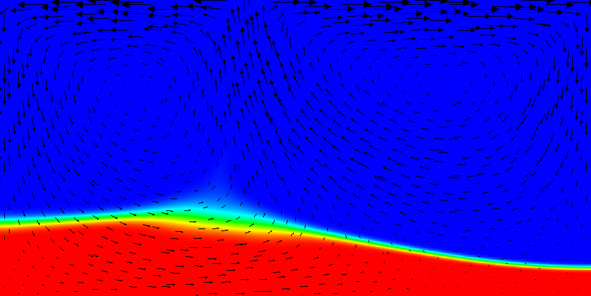
Fig. 37 Active compositional fields: Compositional field 1 at the time t=10. Compared to the results shown in Fig. 33 it is clear that the heavy material stays at the bottom of the domain now. The effect of the density on the velocity field is also clearly visible by noting that at all three times the spreading center at the top boundary is in exactly the same position; this would result in exactly the same velocity field if the density and temperature were constant.

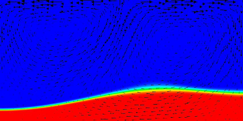
Fig. 38 Active compositional fields: Compositional field 1 at the time t=20. Compared to the results shown in Fig. 33 it is clear that the heavy material stays at the bottom of the domain now. The effect of the density on the velocity field is also clearly visible by noting that at all three times the spreading center at the top boundary is in exactly the same position; this would result in exactly the same velocity field if the density and temperature were constant.

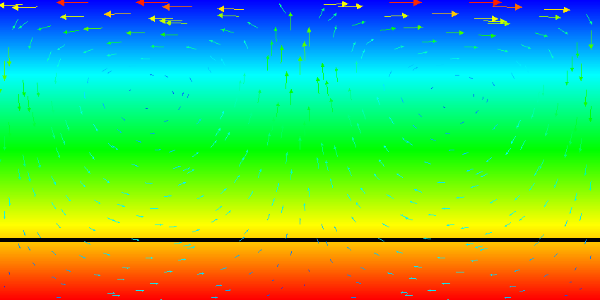
Fig. 39 Active compositional fields: Temperature fields at t=0. The black line is the isocontour line c_1(\mathbf x,t)=0.5 delineating the position of the dense material at the bottom.

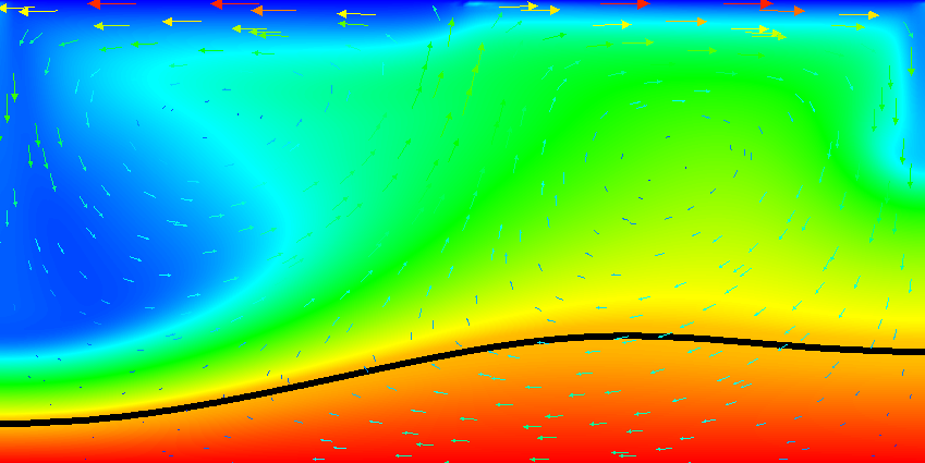
Fig. 40 Active compositional fields: Temperature fields at t=2. The black line is the isocontour line c_1(\mathbf x,t)=0.5 delineating the position of the dense material at the bottom.

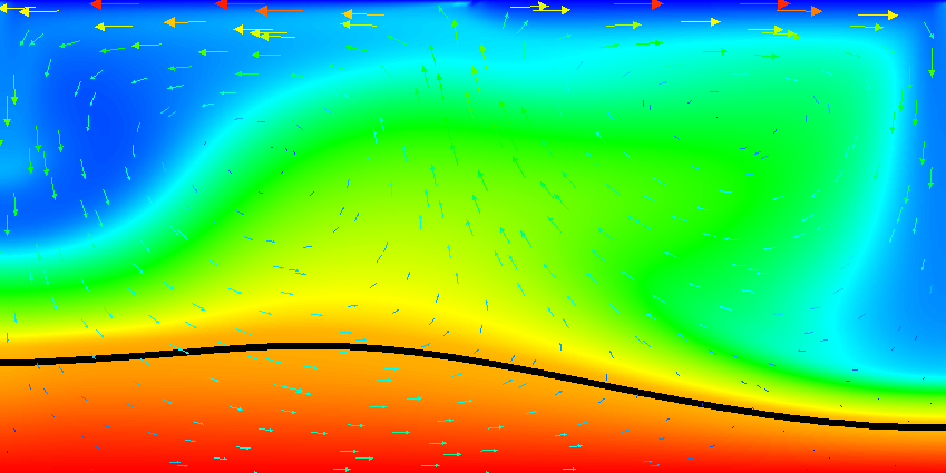
Fig. 41 Active compositional fields: Temperature fields at t=4. The black line is the isocontour line c_1(\mathbf x,t)=0.5 delineating the position of the dense material at the bottom.

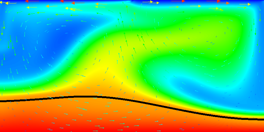
Fig. 42 Active compositional fields: Temperature fields at t=8. The black line is the isocontour line c_1(\mathbf x,t)=0.5 delineating the position of the dense material at the bottom.

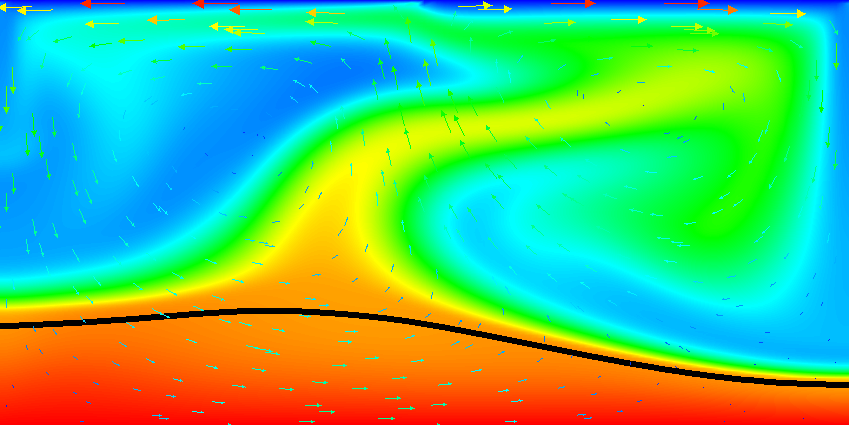
Fig. 43 Active compositional fields: Temperature fields at t=12. The black line is the isocontour line c_1(\mathbf x,t)=0.5 delineating the position of the dense material at the bottom.

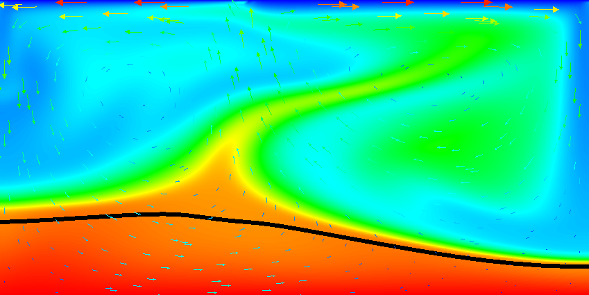
Fig. 44 Active compositional fields: Temperature fields at t=20. The black line is the isocontour line c_1(\mathbf x,t)=0.5 delineating the position of the dense material at the bottom.

Results of this model are visualized in Fig. 36 – Fig. 44 . What is visible is that over the course of the simulation, the material that starts at the bottom of the domain remains there. This can only happen if the circulation is significantly affected by the high density material once the interface starts to become non-horizontal, and this is indeed visible in the velocity vectors. As a second consequence, if the material at the bottom does not move away, then there needs to be a different way for the heat provided at the bottom to get through the bottom layer: either there must be a secondary convection system in the bottom layer, or heat is simply conducted. The pictures in the figure seem to suggest that the latter is the case.

It is easy, using the outline above, to play with the various factors that drive this system, namely:

• The magnitude of the velocity prescribed at the top.

• The magnitude of the velocities induced by thermal buoyancy, as resulting from the magnitude of gravity and the thermal expansion coefficient.

• The magnitude of the velocities induced by compositional variability, as described by the coefficient \(\gamma\) and the magnitude of gravity.

Using the coefficients involved in these considerations, it is trivially possible to map out the parameter space to find which of these effects is dominant. As mentioned in discussing the values in the input file, what is important is the relative size of these parameters, not the fact that currently the density in the material at the bottom is 100 times larger than in the rest of the domain, an effect that from a physical perspective clearly makes no sense at all.

---

1

The actual values do not matter as much here. They are chosen in such a way that the system – previously driven primarily by the velocity boundary conditions at the top – now also feels the impact of the density variations. To have an effect, the buoyancy induced by the density difference between materials must be strong enough to balance or at least approach the forces exerted by whatever is driving the velocity at the top.