Computation of the van Keken Problem with the Volume-of-Fluid Interface Tracking Method

This section is a co-production of Jonathan Robey and E. G. Puckett.

One can also model the van Keken problem with the volume-of-fluid (VOF) interface tracking algorithm in ASPECT. In fact, this problem is particularly well-suited to being computed with the VOF method, since it consists of two distinct, immiscible fluids and interface tracking algorithms are specifically designed not to allow the two fluids to mix. In particular, assuming the computation is sufficiently well-resolved, the fluids will not mix at sub-grid scales over the entire duration of the computation. However, note that this implies that all computations of the van Keken problem made with the VOF method must necessarily be with discontinuous initial conditions. Finally, since one is often interested in a high resolution image of the shape of the interface between the two fluids, one can use the output of the VOF method to examine the interface within individual cells or within regions consisting of groups of cells.

Another advantage the VOF method has over modeling moving interface problems with compositional fields is that for problems in which the interface occupies a relatively small part of the computational domain, all of the computational work in the VOF method is done in cells that lie in a neighborhood of the interface, rather than in the entire computational domain.

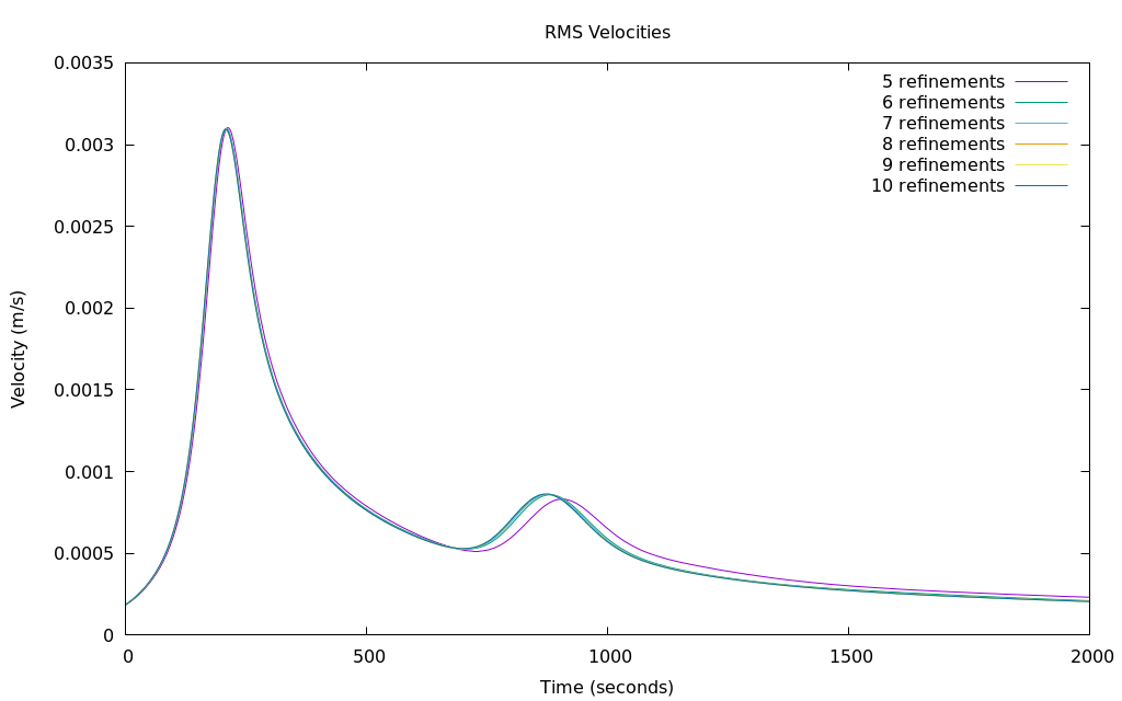
Fig. 132 Evolution of the root mean square velocity as a function of time for computations of the van Keken problem made with the VOF interface tracking algorithm with five different global mesh refinements. Since the VOF initial conditions are discontinuous, the above results should really be compared with the computations with discontinuous initial conditions in Fig. 123. However, the above results also compare extremely favorably with the computations with smoothed, continuous initial conditions for the compositional field in Fig. 124. As in Fig. 124, 5 global refinements correspond to a 32 \(\times\) 32 mesh and 10 global refinements correspond to a 1024 \(\times\) 1024 mesh.

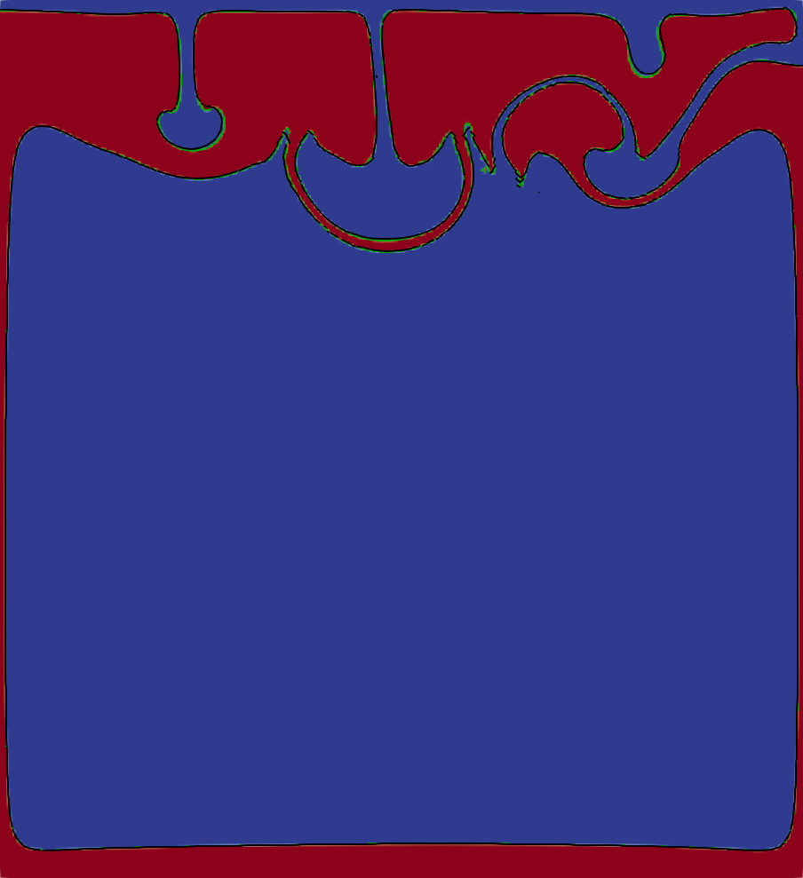
Fig. 133 The results of two computations of the van Keken problem made with the VOF interface tracking algorithm overlaid upon each other at \(t_\text{end}=2000\). This visualization shows the reconstructed boundary between the two materials at the final time \(t_\text{end}\) as computed on a uniform grid with 7 and 8 levels of refinement. The boundaries between the materials are displayed as contours of the fields \(\tilde{\psi}^7(t_\text{end})\) (black) and \(\tilde{\psi}^8\,(t_\text{end})\) (bright green), which are generated by the visualization postprocessor. The contours for the reconstructed material boundaries are superimposed on a color gradient visualization of the material composition for the computation with 8 levels of refinement in order to make the regions with each fluid type more evident. Compare with Fig. 122.

As noted above, when the interface is discontinuous, the van Keken problem is a version of the Rayleigh-Taylor problem, which is unstable to perturbations of all wavelengths whether the two fluids have the same viscosity or different viscosities (e.g. see Chandrasekhar [1961]). Therefore, it is extremely sensitive to the initial conditions. In order to address this sensitivity, we do not use the default approach of computing the initial material volume fractions using a composition quadrature. Instead we compute the initial volume fractions using a signed distance function \(\phi\) as follows [Robey, 2019, Robey and Puckett, 2019].

First we create the function \(\phi\), which has the following two properties: 1) it is positive in the region that contains one of the fluids, which we will refer to as fluid 1, and negative in the complement of this region, which we will refer to as fluid 2, and 2) at each point in the domain the magnitude \(| \phi |\) of \(\phi\) is the distance to the boundary between the two fluids or materials. In the computations shown here, we use an approximation \(\tilde{\phi}\) to \(\phi\) such that the difference between \(\tilde{\phi}\) and \(\phi\) is small enough for the purposes of making the computations high-quality. The use of an approximation as opposed to the function itself is due to obtaining an appropriate function for almost all nontrivial (not a line or a circle) boundaries is extremely difficult. In this case, because the boundary is close to horizontal, we use the vertical distance to the boundary based on the argument that the gradient will not differ sufficiently from \(1\) to induce errors in the initialization computation. The primary advantage of choosing this particular initialization algorithm is that it allows us to more accurately reproduce the initial condition on a sub-grid scale than would otherwise be possible on the coarser grid on which we compute the time evolution of the interface.

subsection Compositional fields
  set Number of fields = 1
  set Compositional field methods = volume of fluid
end

subsection Volume of Fluid
    set Number initialization samples = 16
end

subsection Initial composition model
  set Model name = function
  set Volume of fluid initialization type = C_1:level set

  subsection Function
    set Variable names      = x,z
    set Function constants  = pi=3.1415926
    set Function expression = 0.2+0.02*cos(pi*x/0.9142)-z
  end
end

The relevant sections of the parameter file for this type of initialization of the VOF method appears immediately above. In particular, the combination of Number of initialization samples with the level set initialization type indicates that our initialization will consist of dividing each grid cell into \(16 \times 16\) subcells and the distance to the given initial interface \(f(\mathbf x)\), provided in Function expression, is computed in each of the 256 subcells. We then use this information to compute a piecewise linear interface approximation to \(f(\mathbf x)\). The volume fraction in each subcell is then found in the manner described in Robey [2019], Robey and Puckett [2019]). This initialization procedure provides a much finer and thus, more accurate, initial condition than the standard VOF initialization procedure described above.

While the visualization configuration in a typical parameter file is sufficient for most purposes, when using the VOF method one has the ability to see the division between the fluids reconstructed by the VOF algorithm in each cell. This is accomplished by plotting the zero contour of a field \(\tilde\psi\) that is generated to be \(0\) on the reconstructed interface, positive in the region with fluid 1, and negative in the region with fluid 2. However \(\tilde{\psi}\) does not satisfy the requirement that the magnitude is equal to the distance to the interface as would be required for the signed distance function \(\phi\). The modifications to the parameter file that are necessary in order to draw the reconstructed boundary as a contour are shown immediately below. The full configuration file for this version of the benchmark problem can be found at cookbooks/van-keken-vof/van-keken-vof.prm.

subsection Postprocess
  set List of postprocessors = visualization, velocity statistics
  subsection Visualization
    set List of output variables      = volume of fluid values
    set Output format                 = vtu
    set Time between graphical output = 100
    subsection Volume of Fluid
      set Output interface reconstruction contour = true
    end
  end
end

We made a number of computations of the van Keken problem with the VOF method in order to compare the wall clock times with computations using a DG compositional field. We ran both on the same cluster at global refinements 5–8 using one node with four CPUs and refinements 9 and 10 using two nodes with 16 CPUs. Our results are shown in Table 6. In all of the computations shown in Table 6 we used a CFL number of \(\sigma=0.5\). Due to the change in the CFL number from \(\sigma = 1.0\) in Table 5 to \(\sigma = 0.5\) in Table 6 and the difference between HPC clusters on which the computational results shown in the two tables were made, we can’t make a direct quantitative comparison between the data in Table 5 and Table 6.

However, we can compare the required run time for a VOF computation to that for a DG computation. We note that the use of the VOF advection algorithm significantly reduces the required computation time in all cases, frequently requiring less than half the time required by the DG compositional field.

We now examine the RMS velocity data shown in Fig. 132. Other than for the case of 5 levels of uniform global refinement, the curves for the RMS velocities for \(6\), \(7\), \(8\), \(9\) and \(10\) levels of refinement in Fig. 132 are nearly indistinguishable.

Upon examining the solution at the final time, we note that the general structure of the solution shown in Fig. 133 matches the form and the general structure found in other versions of this benchmark such as in Fig. 122. We also note that the differences in the shape of the interface based on a single refinement as shown in Fig. 133 are minor, although still slightly visible. This is to be expected as refinement is a perturbation of the initial condition at a smaller wave length.

TODO

Table title should contain references, however, Sphinx does not appear to support references in table titles at the moment. Original caption: Comparison of runtimes for the van Keken problem with VOF and a DG compositional field, in which the initial conditions for DG smoothed are as described in The van Keken thermochemical composition benchmark. The times shown are for the full computation, ending at \(t_\text{end} = 2000\) with a CFL number of \(\sigma=0.5\) in both cases. All of these computations were made with ASPECT version 2.2.0-pre (master, commit ef542ecc2) in release mode on the Peloton2 cluster at U.C. Davis. We note that the change in the CFL number \(\sigma\) and the differing choice of cluster makes a direct quantitative comparison between this table and Table 5 invalid due to too many confounding factors.

Table 6 Comparison of runtimes for the van Keken problem with VOF and a DG compositional field, in which the initial conditions for DG smoothed are as described in the previous section. The times shown are for the full computation, ending at \(t_\text{end} = 2000\) with a CFL number of \(\sigma=0.5\) in both cases. All of these computations were made with ASPECT version 2.2.0-pre (master, commit ‘ef542ecc2’) in release mode on the Peloton2 cluster at U.C.Davis. We note that the change in the CFL number \(\sigma\) and the differing choice of cluster makes a direct quantitative comparison between this table and the previous one invalid due to too many confounding factors.

Global Refinement	Number of Processors	VOF	DG
5	4	1.33 minutes	2.57 minutes
6	4	8.51 minutes	19.5 minutes
7	4	1.15 hours	2.49 hours
8	4	8.53 hours	19.6 hours
9	16	16.30 hours	2.72 days
10	16	5.17 days	>6.00 days

The consistency of the results shown here differs noticeably from the behavior of the problem with discontinuous initial conditions when computed with the FEM and DG advection algorithms. One possible reason for these differences is the specialized initialization procedure used for the volume of fluid method, which permits a much more consistent initialization by reducing the variation in the initial condition when the initial mesh is refined.

To study this feature of our algorithm and the sensitivity of the problem to the precise initial condition, we vary the size of the initial interface perturbation and examine the sensitivity of the final results to a small change in the initial conditions. Specifically, we vary the amplitude \(a\) of the cosine function in the initial conditions, as shown below.

subsection Initial composition model
  set Model name = function
  set Volume of fluid initialization type = C_1:level set

  subsection Function
    set Variable names      = x,z
    set Function constants  = pi=3.1415926, a=0.02
    set Function expression = 0.2+a*cos(pi*x/0.9142)-z
  end
end

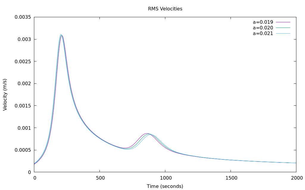
Fig. 134 Computations of the van Keken problem made with the VOF interface tracking algorithm showing the evolution of the RMS velocity as a function of time for small changes in the amplitude a of the cosine function in the initial condition at 7 levels of refinement. Compare to Figures [fig:vk-6] and 1.

In these computations we vary the value of \(a\) from its usual value of \(a = 0.02\) to \(5\% = 0.001\) below its usual value to \(5\%\) above its usual value in increments of \(0.01\). In other words, we compare the values for \(a =0.019\), \(0.020\), and \(0.021\). Upon examination of Fig. 134, we see a visible variation in the location of the second peak, although the overall shape of the curve remains consistent with the curves in Fig. 132. The size of this variation in the initial conditions cannot be expected to be reproduced using the standard compositional quadrature initialization procedure for VOF unless the cell size is on the scale of the change in the value of \(a\); i.e., \(h \, \lessapprox \, \Delta a = 0.001\). We also note that the smoothing parameter which would produce a \(10^{-3}\leq C \leq 1 - 10^{-3}\) band on the order of the same size as the amplitude variation shown here, would be approximately \(2.8 \cdot 10^{-4}\). This perturbation is much smaller than any of the changes in width of the smoothed regions in the computations shown in Fig. 128. In summary, these results demonstrate the sensitivity of the discontinuous version of the van Keken problem to even extremely small variations in the initial conditions.