Two-dimensional models
Contents
Two-dimensional models#
ASPECT allows solving both two- and three-dimensional models via a parameter in the input files, see also Selecting between 2d and 3d. At the same time, the world is unambiguously three-dimensional. This raises the question what exactly we mean when we say that we want to solve two-dimensional problems.
The notion we adopt here - in agreement with that chosen by many other codes - is to think of two-dimensional models in the following way: We assume that the domain we want to solve on is a two-dimensional cross section (parameterized by \(x\) and \(y\) coordinates) that extends infinitely far in both negative and positive \(z\) direction. Further, we assume that the velocity is zero in \(z\) direction and that all variables have no variation in \(z\) direction. As a consequence, we ought to really think of these two-dimensional models as three-dimensional ones in which the \(z\) component of the velocity is zero and so are all \(z\) derivatives.
If one adopts this point of view, the Stokes equations (1)-(2) naturally simplify in a way that allows us to reduce the \(3+1\) equations to only \(2+1\), but it makes clear that the correct description of the compressible strain rate is still \(\varepsilon(\mathbf u) - \frac{1}{3}(\nabla \cdot \mathbf u)\mathbf 1\), rather than using a factor of \(\frac{1}{2}\) for the second term. (A derivation of why the compressible strain rate tensor has this form can be found in Schubert et al. [2001], sec. 6.5.)
It is interesting to realize that this compressible strain rate indeed requires a \(3\times 3\) tensor. While under the assumptions above, we have
with the expected zeros in the last row and column, the full compressible strain rate tensor reads
The entry in the \((3,3)\) position of this tensor may be surprising. It disappears, however, when taking the (three-dimensional) divergence of the stress, as is done in (1), because the divergence applies the \(z\) derivative to all elements of the last row - and the assumption above was that all \(z\) derivatives are zero; consequently, whatever lives in the third row of the strain rate tensor does not matter.
Comments on the final set of equations#
ASPECT solves these equations in essentially the form stated. In particular, the form given in (1) implies that the pressure \(p\) we compute is in fact the total pressure, i.e., the sum of hydrostatic pressure and dynamic pressure (however, see Static or dynamic pressure? for more information on this, as well as the extensive discussion of this issue in Kronbichler et al. [2012]). Consequently, it allows the direct use of this pressure when looking up pressure dependent material parameters.

