The “Stokes’ law” benchmark#

This section was contributed by Juliane Dannberg.

Stokes’ law was derived by George Gabriel Stokes in 1851 and describes the frictional force a sphere with a density different than the surrounding fluid experiences in a laminar flowing viscous medium. A setup for testing this law is a sphere with the radius \(r\) falling in a highly viscous fluid with lower density. Due to its higher density the sphere is accelerated by the gravitational force. While the frictional force increases with the velocity of the falling particle, the buoyancy force remains constant. Thus, after some time the forces will be balanced and the settling velocity of the sphere \(v_s\) will remain constant:

(41)#\[\begin{aligned} \underbrace{6 \pi \, \eta \, r \, v_s}_{\text{frictional force}} = \underbrace{4/3 \pi \, r^3 \, \Delta\rho \, g,}_{\text{buoyancy force}} \end{aligned}\]

where \(\eta\) is the dynamic viscosity of the fluid, \(\Delta\rho\) is the density difference between sphere and fluid and \(g\) the gravitational acceleration. The resulting settling velocity is then given by

(42)#\[\begin{aligned} v_s = \frac{2}{9} \frac{\Delta\rho \, r^2 \, g}{\eta}. \end{aligned}\]

Because we do not take into account inertia in our numerical computation, the falling particle will reach the constant settling velocity right after the first timestep.

For the setup of this benchmark, we chose the following parameters:

(43)#\[\begin{split}\begin{aligned} r &= 200 \, \text{ km}\\ \Delta\rho &= 100 \, \text{ kg/m}^3\\ \eta &= 10^{22} \, \text{ Pa.s}\\ g &= 9.81 \, \text{ m/s}^2. \end{aligned}\end{split}\]

With these values, the exact value of sinking velocity is \(v_s = 8.72\times 10^{-10} \, \text{ m/s}\).

To run this benchmark, we need to set up an input file that describes the situation. In principle, what we need to do is to describe a spherical object with a density that is larger than the surrounding material. There are multiple ways of doing this. For example, we could simply set the initial temperature of the material in the sphere to a lower value, yielding a higher density with any of the common material models. Or, we could use ASPECT’s facilities to advect along what are called “compositional fields” and make the density dependent on these fields.

We will go with the second approach and tell to advect a single compositional field. The initial conditions for this field will be zero outside the sphere and one inside. We then need to also tell the material model to increase the density by \(\Delta\rho=100 \text{ kg m}^{-3}\) times the concentration of the compositional field. This can be done, like everything else, from the input file.

All of this setup is then described by the following input file. (You can find the input file to run this cookbook example in cookbooks/stokes/stokes.prm. For your first runs you will probably want to reduce the number of mesh refinement steps to make things run more quickly.)

############### Global parameters
# We use a 3d setup. Since we are only interested
# in a steady state solution, we set the end time
# equal to the start time to force a single time
# step before the program terminates.

set Dimension                              = 3

set Start time                             = 0
set End time                               = 0
set Use years in output instead of seconds = false

set Output directory                       = output-stokes


############### Parameters describing the model
# The setup is a 3d box with edge length 2890000 in which
# all 6 sides have free slip boundary conditions. Because
# the temperature plays no role in this model we need not
# bother to describe temperature boundary conditions or
# the material parameters that pertain to the temperature.


subsection Geometry model
  set Model name = box

  subsection Box
    set X extent  = 2890000
    set Y extent  = 2890000
    set Z extent  = 2890000
  end
end


subsection Boundary velocity model
  set Tangential velocity boundary indicators = left, right, front, back, bottom, top
end


subsection Material model
  set Model name = simple

  subsection Simple model
    set Reference density             = 3300
    set Viscosity                     = 1e22
  end
end


subsection Gravity model
  set Model name = vertical

  subsection Vertical
    set Magnitude = 9.81
  end
end


############### Parameters describing the temperature field
# As above, there is no need to set anything for the
# temperature boundary conditions.

subsection Initial temperature model
  set Model name = function

  subsection Function
    set Function expression = 0
  end
end

############### Parameters describing the compositional field
# This, however, is the more important part: We need to describe
# the compositional field and its influence on the density
# function. The following blocks say that we want to
# advect a single compositional field and that we give it an
# initial value that is zero outside a sphere of radius
# r=200000m and centered at the point (p,p,p) with
# p=1445000 (which is half the diameter of the box) and one inside.
# The last block re-opens the material model and sets the
# density differential per unit change in compositional field to
# 100.

subsection Compositional fields
  set Number of fields = 1
end

subsection Initial composition model
  set Model name = function

  subsection Function
    set Variable names      = x,y,z
    set Function constants  = r=200000,p=1445000
    set Function expression = if(sqrt((x-p)*(x-p)+(y-p)*(y-p)+(z-p)*(z-p)) > r, 0, 1)
  end
end

subsection Material model
  subsection Simple model
    set Density differential for compositional field 1 = 100
  end
end




############### Parameters describing the discretization
# The following parameters describe how often we want to refine
# the mesh globally and adaptively, what fraction of cells should
# be refined in each adaptive refinement step, and what refinement
# indicator to use when refining the mesh adaptively.

subsection Mesh refinement
  set Initial adaptive refinement        = 4
  set Initial global refinement          = 4
  set Refinement fraction                = 0.2
  set Strategy                           = velocity
end


############### Parameters describing what to do with the solution
# The final section allows us to choose which postprocessors to
# run at the end of each time step. We select to generate graphical
# output that will consist of the primary variables (velocity, pressure,
# temperature and the compositional fields) as well as the density and
# viscosity. We also select to compute some statistics about the
# velocity field.

subsection Postprocess
  set List of postprocessors = visualization, velocity statistics

  subsection Visualization
    set List of output variables = density, viscosity
  end
end

Using this input file, let us try to evaluate the results of the current computations for the settling velocity of the sphere. You can visualize the output in different ways, one of it being ParaView and shown in Fig. 164 (an alternative is to use Visit as described in Visualizing results; 3d images of this simulation using Visit are shown in Fig. 165). Here, ParaView has the advantage that you can calculate the average velocity of the sphere using the following filters:

Threshold (Scalars: C_1, Lower Threshold 0.5, Upper Threshold 1),
Integrate Variables,
Cell Data to Point Data,
Calculator (use the formula sqrt(velocity_x^2+ velocity_y^2+velocity_z^2)/Volume).

If you then look at the Calculator object in the Spreadsheet View, you can see the average sinking velocity of the sphere in the column “Result” and compare it to the theoretical value \(v_s = 8.72\times 10^{-10} \, \text{ m/s}\). In this case, the numerical result is \(8.865\times 10^{-10} \, \text{ m/s}\) when you add a few more refinement steps to actually resolve the 3d flow field adequately. The “velocity statistics” postprocessor we have selected above also provides us with a maximal velocity that is on the same order of magnitude. The difference between the analytical and the numerical values can be explained by different at least the following three points: (i) In our case the sphere is viscous and not rigid as assumed in Stokes’ initial model, leading to a velocity field that varies inside the sphere rather than being constant. (ii) Stokes’ law is derived using an infinite domain but we have a finite box instead. (iii) The mesh may not yet fine enough to provide a fully converges solution. Nevertheless, the fact that we get a result that is accurate to less than 2% is a good indication that implements the equations correctly.

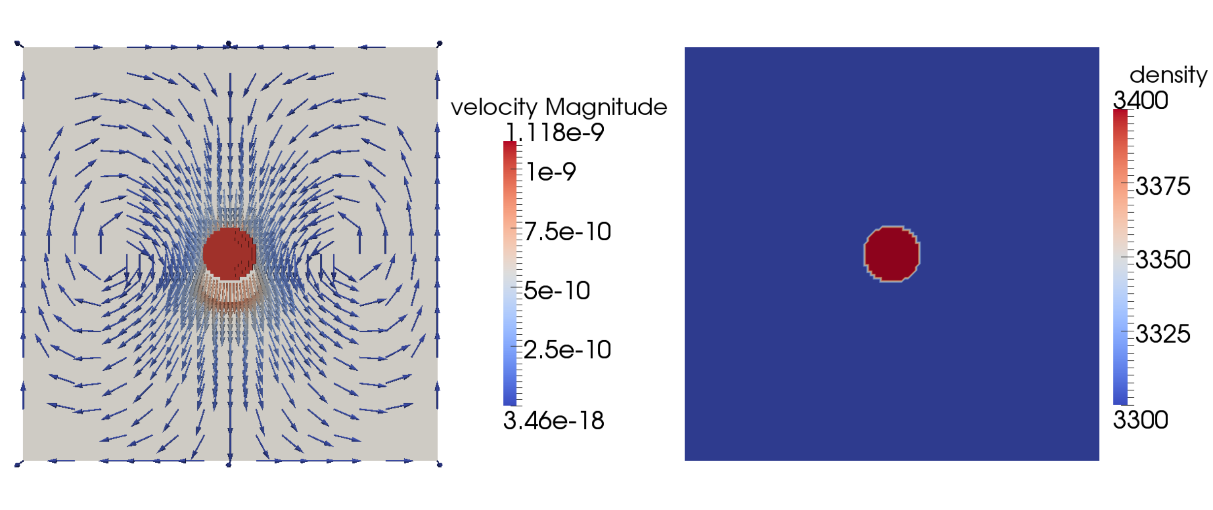
../../../../../_images/stokes2d.png — Fig. 164 Stokes benchmark. Both figures show only a 2D slice of the three-dimensional model. Left: The compositional field and overlaid to it some velocity vectors. The composition is 1 inside a sphere with the radius of 200 km and 0 outside of this sphere. As the velocity vectors show, the sphere sinks in the viscous medium. Right: The density distribution of the model. The compositional density contrast of 100 kg/\text{ m}^3 leads to a higher density inside of the sphere.#

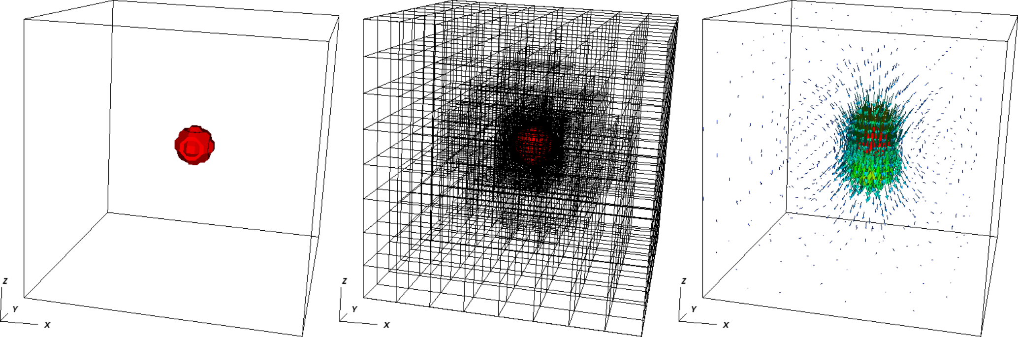
../../../../../_images/stokes3d.png — Fig. 165 Stokes benchmark. Three-dimensional views of the compositional field (left), the adaptively refined mesh (center) and the resulting velocity field (right).#

ASPECT 2.5.0

The “Stokes’ law” benchmark

The “Stokes’ law” benchmark#