Continental extension

This section was contributed by John Naliboff, Anne Glerum, and Valentina Magni

In the crustal deformation examples above, the viscosity depends solely on the Drucker Prager yield criterion defined by the cohesion and internal friction angle. While this approximation works reasonably well for the uppermost crust, deeper portions of the lithosphere may undergo either brittle or viscous deformation, with the latter depending on a combination of composition, temperature, pressure and strain-rate. In effect, a combination of the Drucker-Prager and Diffusion dislocation material models is required. The visco-plastic material model is designed to take into account both brittle (plastic) and non-linear viscous deformation, thus providing a template for modeling complex lithospheric processes. Such a material model can be used in using the following set of input parameters:

subsection Material model
  set Model name = visco plastic
  subsection Visco Plastic

This cookbook provides one such example where the continental lithosphere undergoes extension. Notably, the model design follows that of numerous previously published continental extension studies ([Brune et al., 2014, Huismans and Beaumont, 2011, Naliboff and Buiter, 2015] and references therein)

Continental Extension

The 2D Cartesian model spans 200 (\(x\)) by 100 (\(y\)) km and has a finite element grid with 1.25 and 2.5 km grid spacing, respectively, above and below 50 km depth. This variation in grid spacing is achieved with a single initial adaptive refinement step using the minimum refinement function strategy. Unlike the crustal deformation cookbook (see Crustal deformation), the mesh is not refined with time.

subsection Geometry model
  set Model name = box
  subsection Box
    set X repetitions = 10
    set Y repetitions = 5
    set X extent      = 200e3
    set Y extent      = 100e3
  end
end

subsection Mesh refinement
  set Initial adaptive refinement        = 1
  set Initial global refinement          = 3
  set Time steps between mesh refinement = 0
  set Strategy = minimum refinement function
  subsection Minimum refinement function
    set Coordinate system   = cartesian
    set Variable names      = x,y
    set Function expression = if ( y>=50e3 && x>=40.e3 && x<=160.e3, 4, 3)
  end
end

Similar to the crustal deformation examples above, this model contains a free surface. However, in this example the free surface is advected using the full velocity (e.g., normal projection) rather than only the vertical component. As this projection can lead to significant surface mesh deformation and associated solver convergence issues, diffusion is applied to the free surface at each time step. Deformation is driven by constant horizontal (\(x\)-component) velocities (0.25 cm/yr) on the side boundaries (\(y\)-velocity component unconstrained), while the bottom boundary has vertical inflow to balance the lateral outflow. The top, and bottom boundaries have fixed temperatures, while the sides are insulating. The bottom boundary is also assigned a fixed composition, while the top and sides are unconstrained.

subsection Boundary velocity model
  set Prescribed velocity boundary indicators = left x: function, right x:function, bottom y:function

  subsection Function
    set Variable names      = x,y
    set Function constants  = v=0.0025, w=200.e3, d=100.e3
    set Function expression = if (x < w/2 , -v, v) ; v*2*d/w
  end
end

subsection Mesh deformation
  set Mesh deformation boundary indicators        = top: free surface, top: diffusion
  subsection Free surface
    set Surface velocity projection = normal
  end
  subsection Diffusion
    set Hillslope transport coefficient = 1.e-8
  end
end

subsection Boundary composition model
  set Fixed composition boundary indicators = bottom
  set List of model names = initial composition
end

subsection Boundary temperature model
  set Fixed temperature boundary indicators = bottom, top
  set List of model names = box
  subsection Box
    set Bottom temperature = 1613
    set Top temperature    =  273
  end
end

Sections of the lithosphere with distinct properties are represented by compositional fields for the upper crust (20 km thick), lower crust (20 km thick) and mantle lithosphere (60 km thick). Material (viscous flow law parameters, cohesion, internal friction angle) and thermodynamic properties for each compositional field are based largely on previous numerical studies. Dislocation creep viscous flow parameters are taken from published deformation experiments for wet quartzite ([Rutter and Brodie, 2004]), wet anorthite ([Rybacki et al., 2006]) and dry olivine ([Hirth and Kohlstedt, 2004]). Additional compositional fields are used to track plastic strain and the non-initial plastic strain, with the latter value tracking the same quantity as the plastic strain absent the initial plastic strain values. As discussed further on, the plastic strain is used to soften (e.g., reduce) the friction and cohesion through time based on user-specified bounds and magnitudes. The initial randomized values of plastic strain in the model center localize distributed deformation in this region.

subsection Compositional fields
  set Number of fields = 4
  set Names of fields = upper, lower, mantle, seed
end

subsection Initial composition model
  set Model name = function
  subsection Function
    set Variable names      = x,y
    set Function expression = if(y>=80.e3, 1, 0); \
                              if(y<80.e3 && y>=70.e3, 1, 0); \
                              if(y<70.e3 && y>-100.e3,1, 0); \
                              if(y<68.e3 && y>60.e3 && x>=198.e3 && x<=202.e3 , 1, 0);
  end
end

The initial thermal structure, radiogenic heating model and associated thermal properties are consistent with the prescribed thermal boundary conditions and produce a geotherm characteristic of the continental lithosphere. The equations defining the initial geotherm ([Chapman, 1986]) follow the form

\[\begin{aligned} \label{eq:continental-geotherm-1} T(z) = T_T + \frac{q_T}{k}z - \frac{Az^2}{2k} \end{aligned}\]

where \(T\) is temperature, \(z\) is depth, \(T_T\) is the temperature at the layer surface (top), \(q_T\) is surface heat flux, \(k\) is thermal conductivity, and \(A\) is radiogenic heat production.

For a layer thickness \(\Delta z\), the basal temperature (\(T_B\)) and heat flux (\(q_B\))

\[ \begin{aligned} T_B = T_T + \frac{q_T}{k} \Delta z - \frac{A \Delta z^2}{2k} q_B = q_T - A \Delta z. \end{aligned}\]

In this example, specifying the top (273 \(K\)) temperature, surface heat flow (55 \(mW / m^2\)), thermal conductivity, and radiogenic heat production of each layer provides enough constraints to successively solve for the temperature and heat flux at the top of the lower crust and mantle.

As noted above, the initial zone of randomized plastic strain within the model center and strain softening of the friction and cohesion produces an initial pattern of distributed and unlocalized deformation across the zone of initial plastic strain (Fig. 100). After 5 million years of extension, distributed faulting is clearly evident in both the active and finite deformation fields and surface topography over an approximately 100 km wide region (Fig. 101). While deformation is distributed within this region, the fault system is clearly asymmetric as the rate of deformation and accumulated brittle strain varies between faults. Localization onto the two conjugate rift-bounding border faults is evident from the active deformation field. Notably, deformation of the free surface near the fixed left and right walls is evident at 5 Myr. Continued distortion of the surface mesh near the lateral boundaries may lead to solver issues, which can be overcome by either widening the model or allowing the mesh to deform along these boundaries.

With further extension for millions of years, significant crustal thinning and surface topography development should occur in response to displacement along the rift-bounding faults. However, given that the model only extends to 100 km depth, the simulation will not produce a realistic representation of continental breakup due to the lack of an upwelling asthenosphere layer. Indeed, numerical studies that examine continental breakup, rather than just the initial stages of continental extension, include an asthenospheric layer or modified basal boundary conditions (e.g. Winkler boundary condition in [Brune et al., 2014] for example) as temperature variations associated with lithospheric thinning exert a first-order influence on the deformation patterns. As noted below, numerous additional parameters may also affect the temporal evolution of deformation patterns.

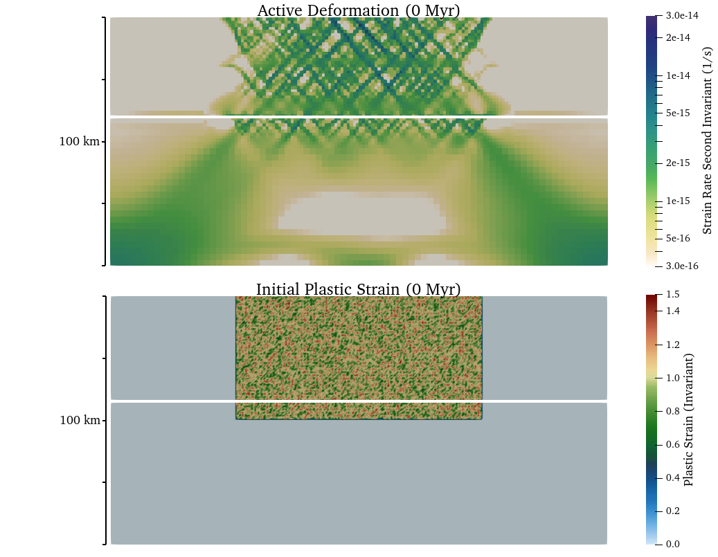
Fig. 100 Initial active deformation field (strain rate second invariant in units of \(s^{-1}\)) and distribution of plastic strain. The white line marks the (893 \(K\)) isotherm (initial Moho temperature).

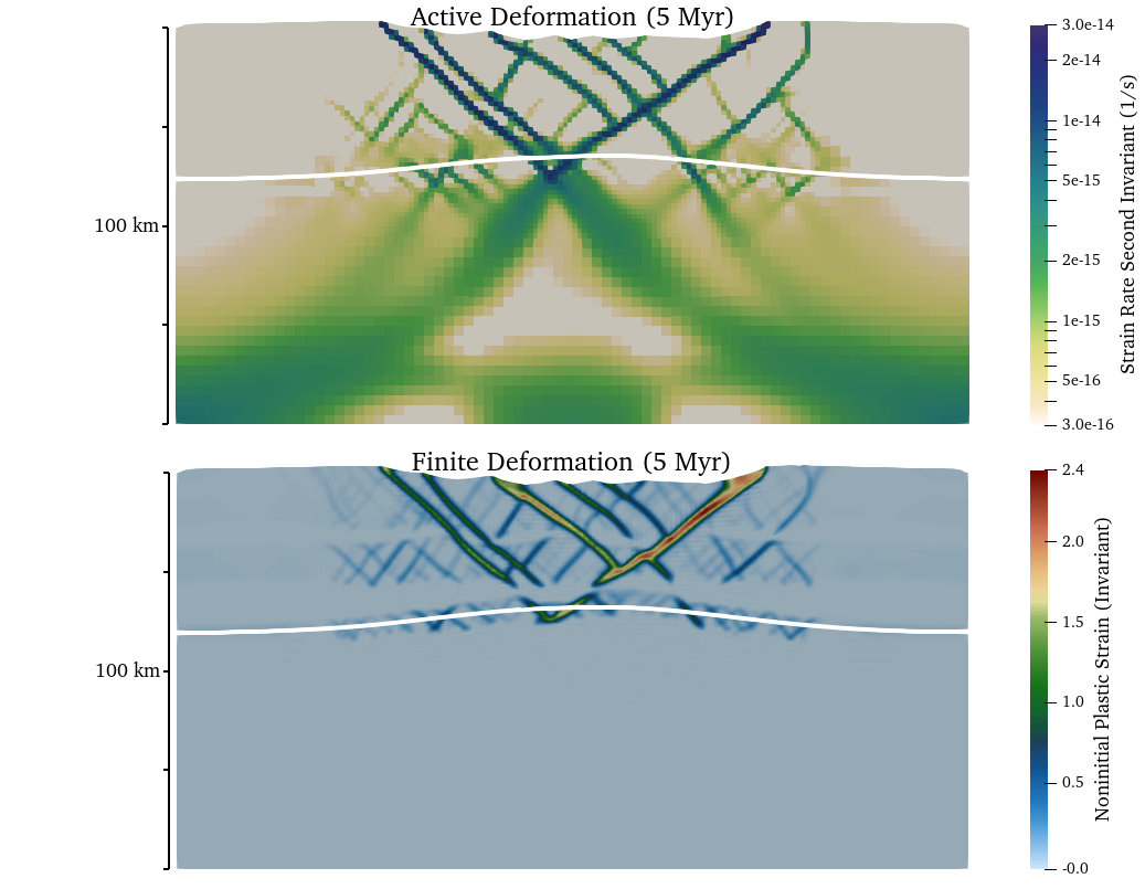
Fig. 101 Active (strain rate second invariant in units of \(s^{-1}\)) and finite (plastic) deformation after 50 million years of extension. The white line marks the (893 \(K\)) isotherm (initial Moho temperature).