The passive case with particles#
In order to advect particles along with the flow field, one just needs to add
the particles postprocessor to the list of postprocessors and specify a few
parameters. We do so in the
cookbooks/composition_passive_particles/composition_passive_particles.prm
input file, which is otherwise just a minor variation of the
cookbooks/composition_passive/composition_passive.prm case discussed in
the previous Section Using passive and active compositional fields. In particular,
the postprocess section now looks like this:
subsection Postprocess
  set List of postprocessors = visualization, particles

  subsection Visualization
    set Time between graphical output = 0.1
  end

  subsection Particles
    set Time between data output = 0.1
    set Data output format       = vtu
  end
end

subsection Particles
  subsection Generator
    subsection Random uniform
      set Number of particles        = 1000
    end
  end
end
The 1000 particles we are asking here are initially uniformly distributed throughout the domain and are, at the end of each time step, advected along with the velocity field just computed. (There are a number of options to decide which method to use for advecting particles, see Subsection: Postprocess / Particles.)
If you run this cookbook, information about all particles will be written into the output directory selected in the input file (as discussed in Section Overview). In the current case, in addition to the files already discussed there, a directory listing at the end of a run will show several particle related files:
aspect> ls -l output/
total 932
-rw-rw-r-- 1 bangerth bangerth  11134 Dec 11 10:08 depth_average.gnuplot
-rw-rw-r-- 1 bangerth bangerth  11294 Dec 11 10:08 log.txt
-rw-rw-r-- 1 bangerth bangerth 326074 Dec 11 10:07 parameters.prm
-rw-rw-r-- 1 bangerth bangerth 577138 Dec 11 10:07 parameters.tex
drwxrwxr-x 2 bangerth bangerth   4096 Dec 11 18:40 particles
-rw-rw-r-- 1 bangerth bangerth    335 Dec 11 18:40 particles.pvd
-rw-rw-r-- 1 bangerth bangerth    168 Dec 11 18:40 particles.visit
drwxr-xr-x 2 bangerth bangerth   4096 Dec 11 10:08 solution
-rw-rw-r-- 1 bangerth bangerth    484 Dec 11 10:08 solution.pvd
-rw-rw-r-- 1 bangerth bangerth    451 Dec 11 10:08 solution.visit
-rw-rw-r-- 1 bangerth bangerth   8267 Dec 11 10:08 statistics
Here, the particles.pvd and particles.visit files contain a list of all
visualization files from all processors and time steps. These files can be
loaded in much the same way as the solution.pvd and solution.visit files
that were discussed in Section Visualizing results. The actual data files
– possibly a large number, but not of much immediate interest to users
– are located in the particles subdirectory.
Coming back to the example at hand, we can visualize the particles that were
advected along by opening both the field-based output files and the ones that
correspond to particles (for example, output/solution.visit and
output/particles.visit) and using a pseudo-color plot for the particles,
selecting the “id” of particles to color each particle. By going
to, for example, the output from the 72nd visualization output, this then
results in a plot like the one shown in Fig. 50.
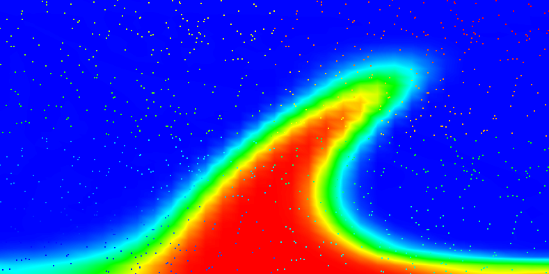
Fig. 50 Passively advected quantities visualized through both a compositional field and a set of 1,000 particles, at t=7.2.#
The particles shown here are not too impressive in still pictures since they are colorized by their particle number, which does not carry any particular meaning other than the fact that it enumerates the particles.[1] The particle “id” can, however, be useful when viewing an animation of time steps. There, the different colors of particles allows the eye to follow the motion of a single particle. This is especially true if, after some time, particles have become well mixed by the flow field and adjacent particles no longer have similar colors. In any case, viewing such animations makes it rather intuitive to understand a flow field, but it can of course not be reproduced in a static medium such as this manual.
In any case, we will see in the next section how to attach more interesting information to particles, and how to visualize these.
Using particle properties.#
The particles in the above example only fulfill the purpose of visualizing the
convection pattern. A more meaningful use for particles is to attach
“properties” to them. A property consists of one or more numbers
(or vectors or tensors) that may either be set at the beginning of the model
run and stay constant, or are updated during the model runtime. These
properties can then be used for many applications, e.g., storing an initial
property (like the position, or initial composition), evaluating a property at
a defined particle path (like the pressure-temperature evolution of a certain
piece of rock), or by integrating a quantity along a particle path (like the
integrated strain a certain domain has experienced). We illustrate these
properties in the cookbook
cookbooks/composition_passive_particles/composition_passive_particles_properties.prm,
in which we add the following lines to the Particles subsection (we also
increase the number of particles compared to the previous section to make the
visualizations below more obvious):
subsection Postprocess
end

subsection Particles
  set List of particle properties = function, initial composition, initial position, pT path

  subsection Function
    set Variable names      = x,y
    set Function expression = if(y<0.2, 1, 0)
  end

  subsection Generator
    subsection Random uniform
      set Number of particles        = 50000
    end
  end
end
These commands make sure that every particle will carry four different
properties (function, pT path, initial position and
initial composition), some of which may be scalars and others can have
multiple components. (A full list of particle properties that can currently be
selected can be found in
Section Subsection: Postprocess / Particles, and new particle
properties can be added as plugins as described in
Section How to write a plugin.) The properties selected above do the
following:
initial position:This particle property simply stores the initial coordinates of the particle and then never changes them. This can be useful to compare the final position of a particle with its initial position and therefore determine how far certain domains traveled during the model runtime. Alternatively, one may want to simply visualize the norm of this vector property (i.e., the norm of the initial position, which is of course equal to the distance from the origin at which a particle started): in mantle simulations in spherical coordinates, the radius is indicative of which part of the mantle a particle comes from, and can therefore be used to visualize where material gets transported over the course of a simulation.initial composition:This property uses the same method to initialize particle properties as is used to initialize the corresponding compositional fields. Using this, it stores the compositional field initialization values at the location where the particle started, and again never changes them. This is useful in the same context as shown for the field-based example in Section Using passive and active compositional fields where we would like to figure where materials ends up. In this case, one would set the initial composition to an indicator function for certain parts of the domain, and then set the initial composition property for the particles to match this composition. Letting the particles advect and at a later time visualizing this particle property will then show where particles came from. In cases where compositional variables undergo changes, e.g., by describing phase changes or chemical reactions, the “initial composition” property can also be useful to compare the final composition of a particle with its initial composition and therefore determine which regions underwent reactions such as those described in Section Using passive and active compositional fields, and where the material that underwent this reaction got transported to.function:This particle property can be used to assign to each particle values that are described based on a function of space. It provides an alternative way to set initial values if you don’t want to first set a compositional field’s initial values based on a function, and then copy these values via the “initial composition” property to particles. In the example above, we use the same function as for the compositional initial composition of field number one in Section Using passive and active compositional fields. Therefore, this property should behave identical to the compositional field (except that the compositional field may have a reaction term that this particle property does not), although the two are of course advected using very different methods. This allows to compare the error in particle position to the numerical diffusion of the compositional field.pT path:This property is interesting in that the particle property’s values always exactly mirror the pressure and temperature at the particle’s current location. This does not seem to be very useful since the information is already available. However, because each particle has a unique id, one can select a particular particle and output its properties (including pressure and temperature based on thepT pathproperty) at all time steps. This allows for the creation of a pressure-temperature curve of a certain piece of rock. This property is interesting in many lithosphere and crustal scale models, because it is determining the metamorphic reactions that happen during deformation processes (e.g., in a subduction zone).
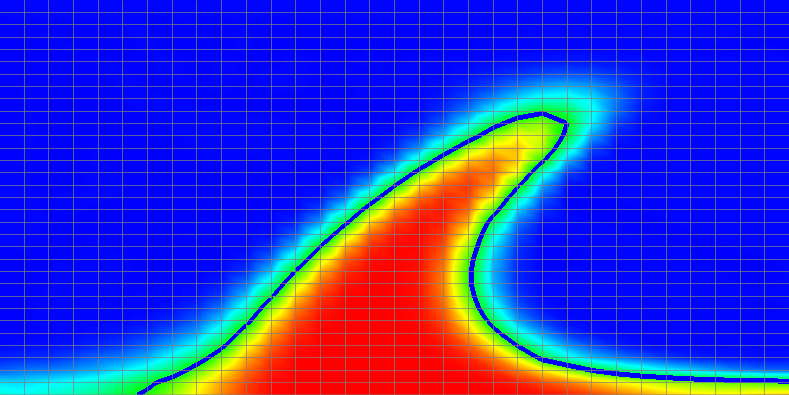
Fig. 51 Passively advected property composition C_1 visualized. The blue line is the 0.5-isocontour for the C_1 field.#
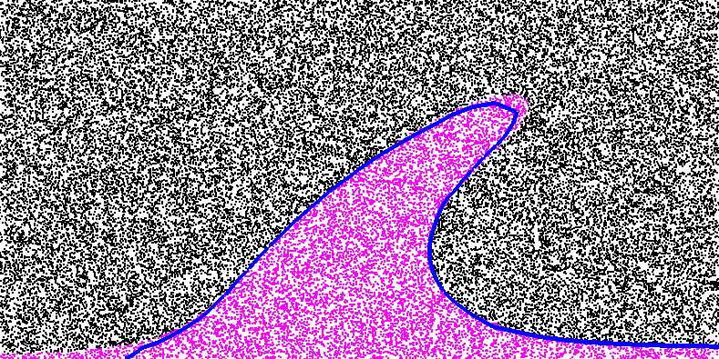
Fig. 52 Passively advected particle property initial C_1 visualized. The blue line is the 0.5-isocontour for the C_1 field.#
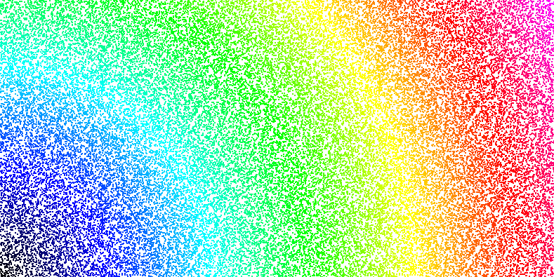
Fig. 53 Passively advected particle properties visualized. Norm of the “initial position” of particles at t=0.#
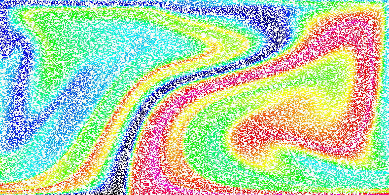
Fig. 54 Passively advected particle properties visualized. Norm of the “initial position” of particles at t=20.#
The results of all of these properties can of course be visualized. Fig. 51 – Fig. 54 shows some of the pictures one can create with particles. The first figures show both the composition field \(C_1\) (along with the mesh on which it is defined) and the corresponding “initial \(C_1\)” particle property, at \(t=7.2\). Because the compositional field does not undergo any reactions, it should of course simply be the initial composition advected along with the flow field, and therefore equal the values of the corresponding particle property. However, field-based compositions suffer from diffusion. On the other hand, the amount of diffusion can easily be decreased by mesh refinement.
The last two figures show the norm of the “initial position” property at the initial time and at time \(t=20\). These images therefore show how far from the origin each of the particles shown was at the initial time.